Semi-volatile organic compounds, or SVOCs for short, are a broad group of moderate volatility substances that possess extremely different chemical characteristics and properties.
These compounds include polybrominated diphenyl ethers (PBDEs), polychlorinated biphenyls (PCBs), pesticides (organophosphorus, organochlorine, nitrogen-based), polycyclic aromatic hydrocarbons (PAHs), phthalates, chloroalkanes, organotin compounds, phenols, and dioxins.
It is known that most SVOCs are environmental pollutants, a few of which continue to persist in the environment for extended periods of time. Today, it is necessary to control organic pollutants in water (groundwater, surface, and drinking) because these pose a serious hazard to aquatic life and may lead to loss of biodiversity. When these pollutants accumulate in the ecosystem, they present a subsequent threat to human health in general.
Therefore, the environmental authorities in many countries across the globe have given due consideration for the assessment of water quality in the recent past. This can be seen by the amendments made to water quality control legislation to feature new regulations containing long lists of controlled substances as well as increasingly rigorous detection limits and quality criteria.
Directive 2013/39/EU[1] — implemented in August 2013 — is part of the EU Water Framework Directive[2] and defines the criteria for the assessment and control of surface water conditions. Amending Directives 2008/105/EC and 2000/60/EC, Directive 2013/39/EU defines a long list of priority substances that need to be tracked within the EU, and also a watch list of substances to be monitored. This current directive thus led to the establishment of Environmental Quality Standards (EQS), with values of pollutant concentration expressed as a maximum allowable concentration (MAC) and as an annual average (AA). In addition, the latest Directive 2015/1787/EU,[3] amending 98/83/EC, defines the analytical criteria for the quality of water for consumption by humans.
Previous regulations defined low (sub-ppt/ppt) detection limits, needing highly sensitive techniques for sufficient ultra-trace analysis. Any developed technique should also be adequately robust so that it can be implemented in process laboratories and can be used for subsequent validation according to established quality standards — ISO 17025 — such that the compliance of the entire process with the said quality criteria can be verified by an independent entity. This is often called the accreditation process.
In this situation, the preceding extraction and/or concentration stage is very important in fulfilling the stipulated detection limits. Most often, this is also the bottleneck of the entire analytical process, which has long been expensive, laborious, lengthy, and detriment for the environment.
Solid phase extraction (SPE) and liquid-liquid extraction (LLE) are examples of commonly used sample preparation methods. These methods are known to be laborious and slow, and need large amounts of samples and solvents (>1 L). SPE cartridges have to be used only once, which further adds to the workflow expense. In addition, both methods create problems with regards to handling the generated wastes.
Eventually, a number of microextraction methods were developed. For instance, solid phase microextraction (SPME) was developed by Janusz Pawliszyn et al. in 1990.[4] Later in 1999, Pat Sandra et al. developed the Stir Bar Sorptive Extraction (SBSE) method based on the same principle as SPME.[5] While both microextraction techniques were better than the traditional methods, they had some drawbacks with respect to routine application and cost.
The new, miniaturized, and ultra-sensitive technique — Bruker μDROP — provides a suitable solution for routine water analysis applications. This method is also fast, affordable, environmentally friendly, and complies with today’s green chemistry recommendations. Moreover, it is based on the principles of Dispersive Liquid-Liquid Microextraction (DLLME), devised by M. Rezaee et al. in 2006.[6] In this innovative microextraction method, three liquid phases are involved, such as water (sample), a water-miscible solvent (dispersant), and a water-immiscible solvent (extractant).
This technique is used to disperse a mist of fine microdroplets of an extractant into the aqueous phase, leading to rapid extraction of analytes. Later, these fine microdroplets become a single microdroplet comprising of all the extracted analytes through centrifugation. Through this technique, high recovery and enrichment factors are effectively obtained. A comparison can be made with the process occurring in electrospray ionization (ESI), in which a mist of microdroplets is generated upon applying an electric field, while dispersive microextraction produces this effect through chemical means via the dispersant.
Subsequent to their development, dispersive microextraction methods have attracted a great deal of interest within the analytical field. In fact, extensive literature on the topic has been published[7] and these methods are used as extraction techniques in numerous instrumental methodologies. Yet, in most of the cases, these techniques have been used only on a certain number of analytes or on one compound class.
The Bruker μDROP technique is the outcome of a proprietary development that enables the concurrent extraction of a large number of analytes from relatively different chemical families. It is possible to determine all SVOCs amenable to GC-MS in just one injection, meeting or surpassing the demands of the most rigorous environmental water analysis regulations.
Experiment
Sample Preparation: Bruker μDROP Method
Figure 1 shows the workflow for sample preparation using the Bruker μDROP technique. With the help of a 40-tube centrifuge, around 40 samples can be prepared in an estimated total time of 10 minutes. Following this stage, all analysis is done automatically and without user interference, with vials being positioned in the gas chromatograph autosampler.
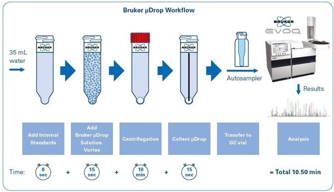
Figure 1. Bruker μDROP workflow for sample preparation.
Individual standards provided by AccuStandard, Inc. (New Haven, CT, USA) were used to prepare the solutions. Dr Ehrenstorfer GmbH (Augsburg, Germany) supplied deuterated internal standards. Table 1 shows Bruker consumables and the general laboratory materials used for sample preparation; Table 2 sums up instrument conditions; Table 4 lists all the analyzed compounds.
Table 1. Laboratory materials and Bruker consumables for sample preparation
| Laboratory Materials |
| Bruker μDROP™ Solvent Extraction Mixture #1 (p/n: 1845184) |
| Bruker μDROP™ Centrifuge Tubes Kit (p/n: 1850435) |
| Centrifuge: Non-refrigerated, minimum speed: 3,000-4,000 rpm |
| Automatic pipettes for liquid handling |
| 2 mL Ultra GCMS vials, screw top wide opening, amber glass with ultra GCMS septa (p/n: 392612016) |
| 200 μL insert, silanized, conical polymer spring (p/n: 392611595) |
Table 2. Mass Spectrometry Method Conditions
| Mass Spectrometer |
Bruker EVOQ GC-TQ MS/MS system |
| |
MS Conditions |
| Ionization |
EI, 70 eV |
| Emission Current |
40 μA |
| Active Focusing Q0 |
135 ºC with Helium |
| Transfer Line Temperature |
280 ºC |
| Source Temperature |
280 ºC |
| CID Gas |
Ar, 2.0 mtorr |
| Detector Mode |
EDR |
| Gas Chromatograph |
Bruker 436 GC |
| |
GC Conditions |
| Injector |
PTV 1079 with programmable temperature |
| Injection Mode |
LVI with solvent vent step |
| Injector Insert |
Siltek 3.4 mm ID Frit gooseneck (p/n: RT217092145) |
| GC Oven Temperature |
Temperature ramp up to 310 ºC |
| GC Column |
Bruker BR-5ms, 30 m x 0.25 mm, 0.25 micron (p/n: BR86377) |
| Carrier Gas |
Helium, 1 mL/min constant flow |
| Total Run Time |
29 min |
| Autosampler |
Bruker 8400 autosampler |
| Software |
Bruker Hystar 4.1/TASQ processing software |
Analytical Method
In total, 59 semi-volatile compounds included under Directive 2013/39/EU were subsequently examined. For quantification purposes, three internal standards were employed — Terbutryn-d5, DDE-4,4′-d8, and Benzo(a)pyrene-d12.
Using the intuitive method editor integrated into the acquisition software, the acquisition method (see Figure 2) was developed in a fast and easy manner. The scan time for each compound in dynamic windows was automatically calculated by the Compound Based Scanning (CBS) software function, thus improving the number of points per peak for accurate quantification (see Figure 3).
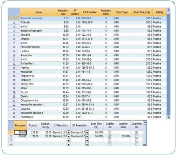
Figure 2. MRM acquisition method.
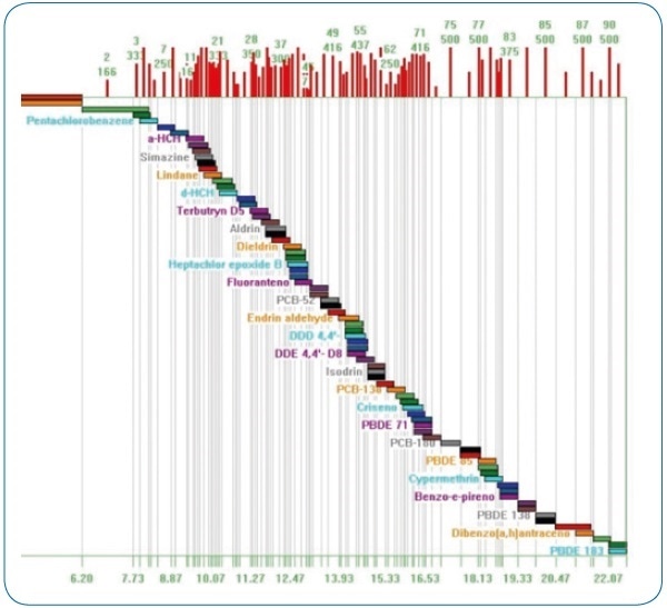
Figure 3. Compound Based Scanning (CBS). Automatic calculation of optimum scan times for each analyzed compound.
When there are no time segments, transitions are assigned to each compound so that any alterations to the acquisition can be automatically edited in the table of compounds, preventing duplication of work and manual editing.
Bruker TASQ
Sample processing as well as statistical calculations of quality parameters was made using Bruker TASQ™ 1.4. Through this software, results can be quickly and comprehensively evaluated (see Figure 4), including the statistical calculations for parameters featured in the validation study.
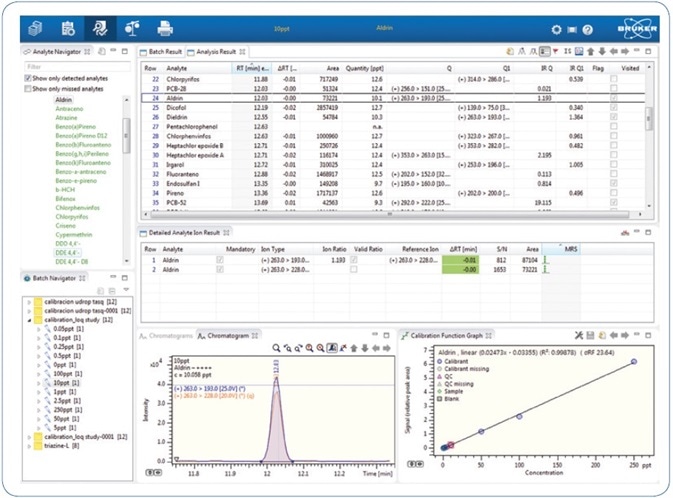
Figure 4. Quick results review using Bruker TASQ 1.4 processing software.
The total ion chromatogram (TIC) of a river water sample, spiked with 10 ppt of the 62 compounds examined, is shown in Figure 5. The tested compounds elute between 7.5 and 22.5 minutes, each presenting a minimum of two transitions (MRM). The scan time is optimized to achieve a minimum of 12 points across every chromatographic peak, in support of fulfilling the validation criteria.
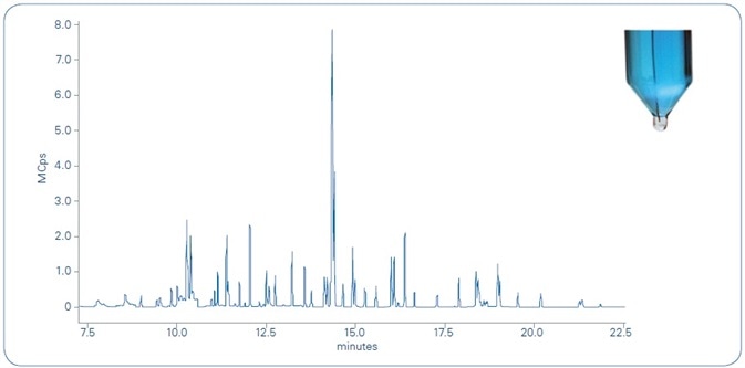
Figure 5. Total ion chromatogram (TIC) of river water sample spiked with 10 ppt of the 62 compounds analyzed. As shown in the photograph in the upper right, the microdroplet (transparent) in the bottom of the tube is clearly distinguishable from the water sample (blue) for easy transfer to the autosampler vial for unattended analysis.
Validation Study
A procedure was followed for method validation. This procedure ensures the results’ quality, applying varied water matrices spiked with the compounds to be examined and covering a broad range of concentrations, beginning with the least concentrations for each compound as defined in Directive 2013/39/EU.
The following are the parameters set for method validation.
Matrices and Blanks: Selectivity
- River water [RIVER] (Eresma River, Segovia, Spain, location: 40°95′44.02″ N; –4°12′11.43″ W)
- Tap water [TAP] (Móstoles, Madrid, Spain, location: 40°20′04.3″ N; 3°52′55.1″ W )
- Sea water [SEA] (Castelldefels, Barcelona, Spain, location: 41°26′32.28″ N; 1°98′57.84″ W)
- Ultrapure water [MQ] (Milli-Q® Quality)
Precision and Accuracy
- RSD (≤30%) of five repetitions from the high and low working range (indicated for each compound listed in Table 4), independent of the matrix. Since procedural standard calibration is used by this method, only the coefficients of variation were evaluated, to be established based on repeat analysis of calibration standards prepared in individual matrices being studied.
Linearity
- The average coefficient of determination (R2 > 0.99) as well as RSD (<30%) of the response factor, obtained from four replicates, independent of the matrix.
Results and Discussion
Linearity
Using the four water matrices under study, the linearity of the technique was evaluated. For individual matrices, solutions of varying concentrations with the 62 examined compounds (deuterated internal standards and analytes) were prepared. Next, each standard sample was extracted after the sample preparation procedure, as shown in Figure 1. For each matrix, each concentration level was separately prepared and extracted in quadruplicate. Thus, four calibration curve repetitions were carried out for each water matrix.
For each analyte, the concentration ranges were set by taking two factors into consideration — calibration curves should have at least five points, and the variation between the low and high working range (coinciding with the curve’s low and high points) should be at least two orders of magnitude. All determinations were carried out on the extracted samples.
The selected low working ranges were invariably less than the minimum parameters defined in Directive 2013/39/EU. Table 3 shows an instance of the quality parameters for Endosulfan. In this case, the low working range was less than 0.5 ppt.
Table 3. Example of Endosulfan concentration levels for different surface waters consistent with Directive 2013/39/EU. “Inland surface waters” covers rivers and lakes. “Other surface waters” includes coastal waters. AA = Annual Average, MAC = Maximum Allowable Concentration.
| Environmental Quality Standards (EQS) for Priority Substances |
| Name of substance |
AA-EQS Inland surface waters (ng/L) |
AA-EQS Other surface waters (ng/L) |
MAC-EQS Inland surface waters (ng/L) |
MAC-EQS Inland surface waters (ng/L) |
| Endosulfan |
5 |
0.5 |
10 |
4 |
The analyzed compounds and the set working ranges are summarized in Table 4. The internal standards (IS) applied for every compound were selected based on structural similarity. Figure 6 shows example calibration curves.
Table 4. Analyzed compounds and set working ranges for calibration using the Bruker μDROP method. Deuterated internal standards are shown in red.
| |
Compounds |
RT (min) |
Low WorkingLevel (ng/L) |
High WorkingLevel (ng/L) |
Internal Standard (IS) |
Calibration Levels (ng/L) |
| 1 |
Pentachlorobenzene |
8.18 |
0.50 |
100 |
DDE-4,4'- d8 |
0.5, 1, 5, 10, 50 and 100 |
| 2 |
Trifluralin |
9.19 |
1.00 |
100 |
DDE-4,4'- d8 |
1, 5, 10, 50 and 100 |
| 3 |
α-HCH |
9.64 |
0.50 |
50 |
DDE-4,4'- d8 |
0.5, 1, 5, 10 and 50 |
| 4 |
Hexachlorobenzene |
9.74 |
0.50 |
50 |
DDE-4,4'- d8 |
0.5, 1, 5, 10 and 50 |
| 5 |
Simazine |
9.93 |
5.00 |
500 |
Terbutryn-d5 |
5, 10, 50, 100, 250 and 500 |
| 6 |
Atrazine |
9.98 |
2.50 |
500 |
Terbutryn-d5 |
2.5, 5, 10, 50, 100, 250 and 500 |
| 7 |
β-HCH |
10.08 |
0.50 |
50 |
DDE-4,4'- d8 |
0.5, 1, 5, 10 and 50 |
| 8 |
γ-HCH (Lindane) |
10.20 |
0.50 |
50 |
DDE-4,4'- d8 |
0.5, 1, 5, 10 and 50 |
| 9 |
Anthracene |
10.60 |
2.50 |
250 |
Benzo-(a)-pyrene- d12 |
2.5, 5, 10, 50, 100 and 250 |
| 10 |
δ-HCH |
10.68 |
0.50 |
50 |
DDE-4,4'- d8 |
0.5, 1, 5, 10 and 50 |
| 11 |
Alachlor |
11.26 |
1.00 |
50 |
DDE-4,4'- d8 |
1, 5, 10, 50 and 50 |
| 12 |
Heptachlor |
11.45 |
0.10 |
50 |
DDE-4,4'- d8 |
0.1, 0.25, 0.5, 1, 5, 10 and 50 |
| 13 |
Terbutryn-d5 (IS) |
11.79 |
- |
- |
- |
10 for all calibration levels |
| 14 |
Terbutryn |
11.83 |
0.50 |
50 |
Terbutryn-d5 |
0.5, 1, 5, 10 and 50 |
| 15 |
Chlorpyrifos |
11.95 |
1.00 |
100 |
DDE-4,4'- d8 |
1, 5, 10, 50 and 100 |
| 16 |
Aldrin |
12.09 |
0.50 |
50 |
DDE-4,4'- d8 |
0.5, 1, 5, 10 and 50 |
| 17 |
Dicofol |
12.25 |
0.10 |
50 |
DDE-4,4'- d8 |
0.1, 0.25, 0.5, 1, 5, 10 and 50 |
| 18 |
Isodrin |
12.61 |
0.50 |
50 |
DDE-4,4'- d8 |
0.5, 1, 5, 10 and 50 |
| 19 |
Chlorfenvinfos |
12.71 |
1.00 |
250 |
DDE-4,4'- d8 |
1, 5, 10, 50, 100 and 250 |
| 20 |
Heptachlor epoxide B |
12.77 |
0.10 |
50 |
DDE-4,4'- d8 |
0.1, 0.25, 0.5, 1, 5, 10 and 50 |
| 21 |
Heptachlor epoxide A |
12.87 |
0.10 |
50 |
DDE-4,4'- d8 |
0.1, 0.25, 0.5, 1, 5, 10 and 50 |
| 22 |
Cibutryn |
12.89 |
0.25 |
50 |
DDE-4,4'- d8 |
0.25, 0.5, 1, 5, 10 and 50 |
| 23 |
Fluoranthene |
12.96 |
1.00 |
100 |
Benzo-(a)-pyrene- d12 |
1, 5, 10, 50 and 100 |
| 24 |
Endosulfan I |
13.42 |
0.25 |
50 |
DDE-4,4'- d8 |
0.25, 0.5, 1, 5, 10 and 50 |
| 25 |
DDE-4,4'- d8 (IS) |
13.73 |
- |
- |
- |
10 for all calibration levels |
| 26 |
DDE-4,4' |
13.77 |
0.50 |
100 |
DDE-4,4'- d8 |
0.5, 1, 5, 10, 50 and 100 |
| 27 |
Dieldrin |
13.92 |
0.50 |
50 |
DDE-4,4'- d8 |
0.5, 1, 5, 10 and 50 |
| 28 |
PCB81 |
13.98 |
0.10 |
50 |
DDE-4,4'- d8 |
0.1, 0.5, 1, 5, 10 and 50 |
| 29 |
Endrin |
14.30 |
0.50 |
50 |
DDE-4,4'- d8 |
0.5, 1, 5, 10 and 50 |
| 30 |
PCB77 |
14.35 |
0.10 |
50 |
DDE-4,4'- d8 |
0.1, 0.5, 1, 5, 10 and 50 |
| 31 |
Endosulfan II |
14.50 |
0.25 |
50 |
DDE-4,4'- d8 |
0.25, 0.5, 1, 5, 10 and 50 |
| 32 |
PCB126 |
14.51 |
0.10 |
50 |
DDE-4,4'- d8 |
0.1, 0.5, 1, 5, 10 and 50 |
| 33 |
PCB123 |
14.54 |
0.10 |
50 |
DDE-4,4'- d8 |
0.1, 0.5, 1, 5, 10 and 50 |
| 34 |
PBDE 28 |
14.55 |
0.10 |
50 |
DDE-4,4'- d8 |
0.1, 0.5, 1, 5, 10 and 50 |
| 35 |
DDD- 4,4' |
14.55 |
0.50 |
100 |
DDE-4,4'- d8 |
0.5, 1, 5, 10, 50 and 100 |
| 36 |
DDT- 2,4' |
14.58 |
0.50 |
100 |
DDE-4,4'- d8 |
0.5, 1, 5, 10, 50 and 100 |
| 37 |
PCB118 |
14.76 |
0.10 |
50 |
DDE-4,4'- d8 |
0.1, 0.5, 1, 5, 10 and 50 |
| 38 |
Aclonifen |
14.80 |
1.00 |
100 |
DDE-4,4'- d8 |
1, 2.5, 5, 10, 50 and 100 |
| 39 |
PCB114 |
14.90 |
0.10 |
50 |
DDE-4,4'- d8 |
0.1, 0.5, 1, 5, 10 and 50 |
| 40 |
Quinoxyfen |
15.03 |
0.50 |
50 |
DDE-4,4'- d8 |
0.5, 1, 5, 10 and 50 |
| 41 |
Endosulfan Sulfate |
15.18 |
0.25 |
50 |
DDE-4,4'- d8 |
0.25, 0.5, 1, 5, 10 and 50 |
| 42 |
DDT- 4,4' |
15.21 |
0.50 |
100 |
DDE-4,4'- d8 |
0.5, 1, 5, 10, 50 and 100 |
| 43 |
PCB105 |
15.43 |
0.10 |
50 |
DDE-4,4'- d8 |
0.1, 0.5, 1, 5, 10 and 50 |
| 44 |
PCB167 |
15.51 |
0.10 |
50 |
DDE-4,4'- d8 |
0.1, 0.5, 1, 5, 10 and 50 |
| 45 |
Bifenox |
16.37 |
0.25 |
50 |
DDE-4,4'- d8 |
0.25, 0.5, 1, 5, 10 and 50 |
| 46 |
PCB169 |
16.55 |
0.10 |
50 |
DDE-4,4'- d8 |
0.1, 0.5, 1, 5, 10 and 50 |
| 47 |
PCB156 |
16.62 |
0.10 |
50 |
DDE-4,4'- d8 |
0.1, 0.5, 1, 5, 10 and 50 |
| 48 |
PBDE 47 |
16.74 |
0.10 |
50 |
DDE-4,4'- d8 |
0.1, 0.25, 0.5, 1, 5, 10 and 50 |
| 49 |
PCB157 |
16.84 |
0.10 |
50 |
DDE-4,4'- d8 |
0.1, 0.5, 1, 5, 10 and 50 |
| 50 |
PCB189 |
17.05 |
0.10 |
50 |
DDE-4,4'- d8 |
0.1, 0.5, 1, 5, 10 and 50 |
| 51 |
PBDE 100 |
17.58 |
0.10 |
50 |
DDE-4,4'- d8 |
0.1, 0.25, 0.5, 1, 5, 10 and 50 |
| 52 |
PBDE 99 |
17.85 |
0.10 |
50 |
DDE-4,4'- d8 |
0.1, 0.25, 0.5, 1, 5, 10 and 50 |
| 53 |
Benzo(b)fluoranthene |
18.58 |
0.25 |
50 |
Benzo-(a)-pyrene- d12 |
0.25, 0.5, 1, 5, 10 and 50 |
| 54 |
Benzo(k)fluoranthene |
18.64 |
0.25 |
50 |
Benzo-(a)-pyrene- d12 |
0.25, 0.5, 1, 5, 10 and 50 |
| 55 |
Cypermethrin |
18.72 |
0.25 |
50 |
Benzo-(a)-pyrene- d12 |
0.25, 0.5, 1, 5, 10 and 50 |
| 56 |
Benzo(a)pyrene-d12 (IS) |
19.15 |
- |
- |
- |
1 for all calibration levels |
| 57 |
Benzo(a)pyrene |
19.24 |
0.10 |
50 |
Benzo-(a)-pyrene- d12 |
0.1, 0.25, 0.5, 1, 5, 10 and 50 |
| 58 |
PBDE 154 |
19.64 |
0.10 |
50 |
DDE-4,4'- d8 |
0.1, 0.25, 0.5, 1, 5, 10 and 50 |
| 59 |
PBDE 153 |
19.78 |
0.10 |
50 |
DDE-4,4'- d8 |
0.1, 0.25, 0.5, 1, 5, 10 and 50 |
| 60 |
Indene(1,2,3-c,d)pyrene |
21.53 |
0.50 |
50 |
Benzo-(a)-pyrene- d12 |
0.5, 1, 5, 10 and 50 |
| 61 |
Dibenzo(a,h)anthracene |
21.56 |
0.50 |
50 |
Benzo-(a)-pyrene- d12 |
0.5, 1, 5, 10 and 50 |
| 62 |
Benzo(g,h,i)perylene |
22.13 |
0.50 |
50 |
Benzo-(a)-pyrene- d12 |
0.5, 1, 5, 10 and 50 |
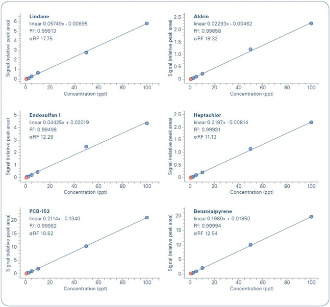
Figure 6. Examples of calibration curves for analyzed compounds.
The outcomes of the linearity study of the calibration curves, for each analyzed compound in each water sample, are shown in Figure 7. As demonstrated, the formerly set quality criteria are met in all cases—R2 ≥ 0.99, with a difference (RSD %) of the curve’s response factor ≤ 30% (σRF) for the whole concentration range being studied.
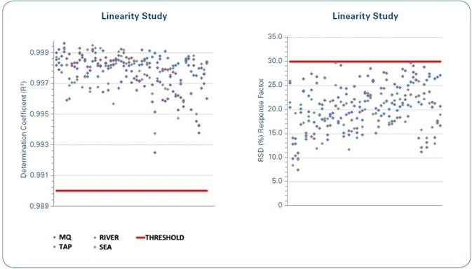
Figure 7. Linearity study: The red lines indicate the limits for the set quality criteria. Left: Coefficient of determination (R2) of the calibration curves of each compound for each of the water matrices under study. Right: Relative Standard Deviation (RSD%) of the response factor for the calibration curves of each compound for each of the water matrices under study.
A number of relevant analytics are revealed by the linearity study data. The first is that 90% of the achieved coefficients of determination (R2) are above 0.995. This implies that consideration might be given to make this criterion more limited if stipulated by legislation.
According to the response factor variation (RSD%), most of the values are grouped together from 10% to 30%. In such a case, the earlier set criterion is modified to match with the analytical reality.
Matrix Effect
Another important aspect to be noted is that with the Bruker μDROP technique, matrix effects become irrelevant for all matrices being studied, enabling a routine application for extremely different water samples.
Matrix effects were assessed by taking the slope of the calibration curve for MQ water as a reference and comparing it against the slope of the calibration curves for other water samples (SEA, TAP, and RIVER), as shown in Figure 8.
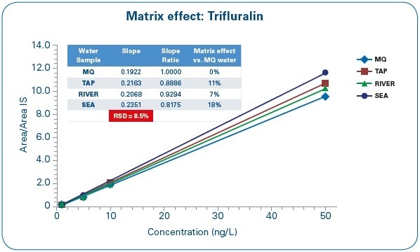
Figure 8. Matrix Effect Assessment: Trifluralin calibration curves in different water matrices.
The variation between the calibration curve slopes differs between 7% and 18%, and the difference coefficient between the slope values is 8.5%. Based on these results, the laboratory can measure sea, tap, or river water samples through a calibration curve prepared with pure water.
Precision and Accuracy
As established before, precision was evaluated by finding out the dispersal (RSD %) of five repetitions of each water sample being analyzed, taken by four entirely different operators over five different days (inter-day precision). Next, precision was established for the high and low working level for each of the samples. All determinations were carried out on extracted samples, the outcomes of which are illustrated in Figure 9.
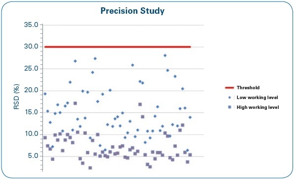
Figure 9. Precision study: RSD (%) of four repetitions at low and high working levels for each of the water samples under study.
From the set of results summed up in Figure 9, it can be seen that no RSD (%) average value surpasses the 30% set as the acceptance criterion, and as might be anticipated, low working ranges provide less precision when compared to high ranges. Most of the RSD data are within the 5%–20% range.
With regards to the accuracy, as observed before, this technique applies calibration through the extraction of patterns introduced to the matrix (“procedural standard calibration”). Instead of determining the recoveries in each matrix, the coefficient of variation of frequent analysis of calibration standards formulated in each matrix under analysis is determined once again.
Sensitivity: Method Reporting Limit (MRL) and Method Detection Limit (MDL)
Traditionally, limits of detection have been calculated using the mean of the signal-to-noise (S/N) ratio for a chromatographic peak in relation to the background of a blank sample and subsequently using different statistical calculations.
Yet, extremely low background, with near-zero values, are generated for many transitions by latest GC-triple quadrupole MS/MS systems, working in MRM mode. Apparently, any statistical calculation with near-zero values creates wrong estimates of limits of detection that are beyond the analytical reality. As a result, there has been a considerable amount of confusion when it comes to defining the limits of detection, and presently published literature unfortunately contains different definitions, nomenclatures, and concepts.[8]
Another challenge faced in the field of multi-residue analysis of considerably different matrices is that a fully blank matrix sample is usually not available. Therefore, in this analysis, the following two parameters were used to experimentally establish method sensitivity:
- Method Reporting Limit or MRL: This is defined as the lowest concentration that can be consistently measured to fulfill the set accuracy and precision criteria. Essentially, in this study, the values relating to the initial calibration point contained in the method validation are set as MRLs—to put it in simpler terms, the low working level for each of the compounds shown in Table 4.
- Method Detection Limit or MDL: This is defined as the least detected concentration of a compound, taking sample preparation and the particular method parameters into consideration. For every compound, the quantification as well as confirmation ions should be detected with a S/N of greater than 10.
Extracted water samples spiked with reducing analyte concentrations were prepared to establish the MDLs. After each analysis, a blank sample was injected, which was subjected to the same extraction procedure.
Next, the MDLs of individual compounds were set comparing the least concentration at which the compound can be detected against the relative blank. In this fashion, realistic MDLs were determined. Very low estimates prepared using statistical calculations of the S/N could result in false positives in regular applications.
Table 5 shows the outcomes of the MDL and MRL values for all of the analyzed compounds.
Table 5. The Method Reporting Limits (MRLs) and Method Detection Limits (MDLs) for all analyzed compounds. Values not applicable (n/a) for internal standards.
| |
Compounds |
MRL (ng/L) |
MDL (ng/L) |
| 1 |
Pentachlorobenzene |
0.50 |
0.20 |
| 2 |
Trifluralin |
1.00 |
0.05 |
| 3 |
α-HCH |
0.50 |
0.10 |
| 4 |
Hexachlorobenzene |
0.50 |
0.10 |
| 5 |
Simazine |
5.00 |
2.50 |
| 6 |
Atrazine |
2.50 |
1.00 |
| 7 |
β-HCH |
0.50 |
0.10 |
| 8 |
γ-HCH (Lindane) |
0.50 |
0.10 |
| 9 |
Anthracene |
2.50 |
0.05 |
| 10 |
δ-HCH |
0.50 |
0.10 |
| 11 |
Alachlor |
1.00 |
0.10 |
| 12 |
Heptachlor |
0.10 |
0.05 |
| 13 |
Terbutryn-d5 (IS) |
n/a |
n/a |
| 14 |
Terbutryn |
0.50 |
0.05 |
| 15 |
Chlorpyrifos |
1.00 |
0.05 |
| 16 |
Aldrin |
0.50 |
0.25 |
| 17 |
Dicofol |
0.10 |
0.02 |
| 18 |
Isodrin |
0.50 |
0.20 |
| 19 |
Chlorfenvinfos |
1.00 |
0.05 |
| 20 |
Heptachlor epoxide B |
0.10 |
0.05 |
| 21 |
Heptachlor epoxide A |
0.10 |
0.05 |
| 22 |
Cibutryn |
0.50 |
0.25 |
| 23 |
Fluoranthene |
1.00 |
0.25 |
| 24 |
Endosulfan I |
0.25 |
0.10 |
| 25 |
DDE-4,4'- d8 (IS) |
n/a |
n/a |
| 26 |
DDE-4,4' |
0.50 |
0.10 |
| 27 |
Dieldrin |
0.50 |
0.10 |
| 28 |
PCB81 |
0.10 |
0.05 |
| 29 |
Endrin |
0.50 |
0.10 |
| 30 |
PCB77 |
0.10 |
0.05 |
| 31 |
Endosulfan II |
0.25 |
0.10 |
| 32 |
PCB126 |
0.10 |
0.05 |
| 33 |
PCB123 |
0.10 |
0.05 |
| 34 |
PBDE 28 |
0.10 |
0.05 |
| 35 |
DDD- 4,4' |
0.50 |
0.05 |
| 36 |
DDT- 2,4' |
0.50 |
0.05 |
| 37 |
PCB118 |
0.10 |
0.05 |
| 38 |
Aclonifen |
2.50 |
1.00 |
| 39 |
PCB114 |
0.10 |
0.05 |
| 40 |
Quinoxyfen |
0.50 |
0.25 |
| 41 |
Endosulfan Sulfate |
0.25 |
0.05 |
| 42 |
DDT- 4,4' |
0.50 |
0.05 |
| 43 |
PCB105 |
0.10 |
0.05 |
| 44 |
PCB167 |
0.10 |
0.05 |
| 45 |
Bifenox |
0.25 |
0.10 |
| 46 |
PCB169 |
0.10 |
0.05 |
| 47 |
PCB156 |
0.10 |
0.05 |
| 48 |
PBDE 47 |
0.10 |
0.05 |
| 49 |
PCB157 |
0.10 |
0.05 |
| 50 |
PCB189 |
0.10 |
0.05 |
| 51 |
PBDE 100 |
0.10 |
0.05 |
| 52 |
PBDE 99 |
0.10 |
0.05 |
| 53 |
Benzo(b)fluoranthene |
0.25 |
0.05 |
| 54 |
Benzo(k)fluoranthene |
0.25 |
0.05 |
| 55 |
Cypermethrin |
0.25 |
0.05 |
| 56 |
Benzo(a)pyrene-d12 (IS) |
n/a |
n/a |
| 57 |
Benzo(a)pyrene |
0.10 |
0.05 |
| 58 |
PBDE 154 |
0.10 |
0.05 |
| 59 |
PBDE 153 |
0.10 |
0.05 |
| 60 |
Indene(1,2,3-c,d)pyrene |
0.50 |
0.10 |
| 61 |
Dibenzo(a,h)anthracene |
0.50 |
0.10 |
| 62 |
Benzo(g,h,i)perylene |
0.50 |
0.10 |
The relative chromatograms for the set MRL and MDL levels for chlorfenvinphos are shown in Figure 10, demonstrating the quantification and confirmation ions for both levels. Both these show an S/N > 10 for the MDL level.
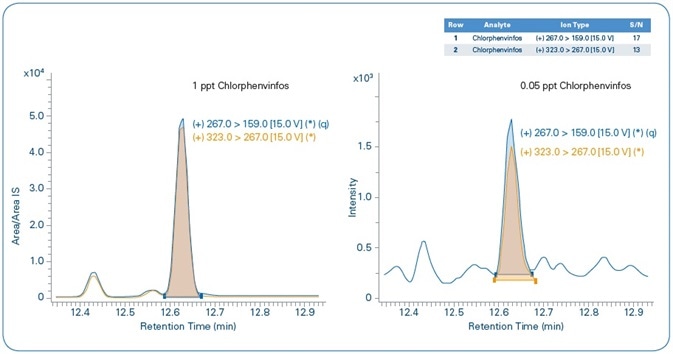
Figure 10. Chlorfenvinphos: MRL = 1 ppt (left), MDL=0.05 ppt (right). Blue = quantification ion, Orange = confirmation ion.
Figure 11 shows the chromatograms for the MDL levels of select compounds when compared to the corresponding blank samples. In all the cases, both quantification and confirmation ions can be noted. Although compounds are not detected in the majority of the corresponding blank samples, traces of PBDE 47, Benzo(a)pyrene, and Endosulfan II are detected in the corresponding blank samples but in concentrations that are much below their set MDL levels.
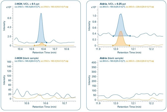
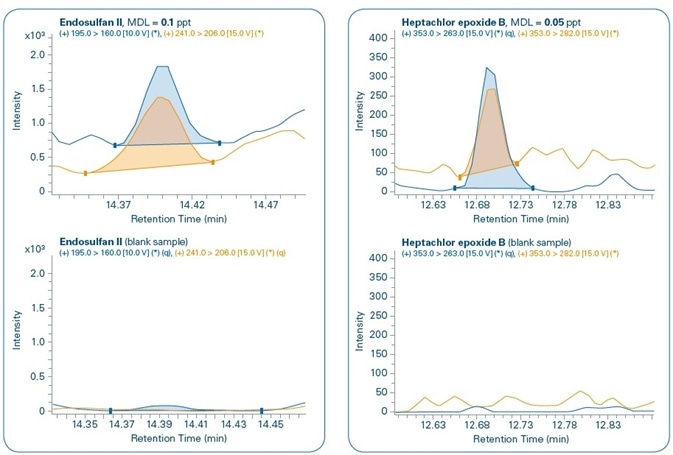
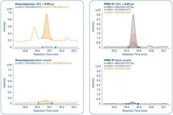
Figure 11. Sensitivity study. Chromatograms of different compounds at the method detection limit (MDL) set for each compound and comparison with corresponding blank samples. Quantification (q) and confirmation ions can be seen for all compounds.
It can be concluded from the sensitivity study that both MDLs and MRLs were achieved at sub-ppt and low-ppt levels for all examined compounds, with validated and realistic limits for routine application of the technique.
Conclusion
The Bruker μDROP methodology provides a fast and dependable solution for quality control of water and surface water for consumption by humans. This method is perfect for high productivity and routine application in environmental laboratories, and allows ultra-sensitive determination of semi-volatile organic compounds down to sub-ppt and low-ppt levels through a reduced volume of sample (35 mL).
The Bruker μDROP method — based on the recent miniaturized microextraction techniques — not only provides low per-sample cost but also reduces environmental impact in the creation and management of lab waste.
With the help of Bruker’s robust EVOQ GC-TQ MS/MS system, the technique was verified using extractions and matrices with different operators, resulting in excellent accuracy, precision, and linearity values to conform to the analytical criteria defined in the present European directives on water policy.
References
[1] http://eur-lex.europa.eu/legal-content/EN/TXT/PDF/?uri=CELEX:32013L0039: Directive 2013/39/ EU of 12 August 2013 amending Directives 2000/60/EC and 2008/105/EC as regards priority substances in the field of water policy.
[2] http://ec.europa.eu/environment/water/water-framework/index_en.html: Directive 2000/60/EC of 23 October 2000 establishing a framework for Community action in the field of water policy.
[3] http://eur-lex.europa.eu/legal-content/EN/TXT/PDF/?uri=CELEX:32015L1787: Commission Directive (EU) 2015/1787 of 6 October 2015 amending Annexes II and III to Council Directive 98/83/EC on the quality of water intended for human consumption.
[4] Arthur, C.L., Pawliszyn, J. (1990) Solid phase microextraction with thermal desorption using fused silica optical fibers. Anal. Chem., 62:2145–2148.
[5] Baltussen, E., Sandra, P., David, F., and Cramers, C.A. (1999) Stir bar sorptive extraction (SBSE), a novel extraction technique for aqueous samples: Theory and principles. J. Microcolumn Sep., 11: 737–747.
[6] Rezaee, M., Assadi, Y., Milani, M.R., Aghaee, E., Ahmadi, F., Berijani, S. (2006) Determination of organic compounds in water using dispersive liquid-liquid microextraction. Journal of Chromatography A, 1116: 1–9.
[7] Yan H., Wang, H., (2013) Recent development and applications of dispersive liquid–liquid microextraction. Journal of Chromatography A, 1295: 1– 15.
[8] Wenzl, T., Haedrich, J., Schaechtele, A., Robouch, P., Stroka, J. (2016) European Commission: JRC Technical Reports, Guidance Document on the Estimation of LOD and LOQ for Measurements in the Field of Contaminants in Feed and Food. https://ec.europa.eu/jrc
About Bruker Life Sciences Mass Spectrometry

Discover new ways to apply mass spectrometry to today’s most pressing analytical challenges. Innovations such as Trapped Ion Mobility (TIMS), smartbeam and scanning lasers for MALDI-MS Imaging that deliver true pixel fidelity, and eXtreme Resolution FTMS (XR) technology capable to reveal Isotopic Fine Structure (IFS) signatures are pushing scientific exploration to new heights. Bruker's mass spectrometry solutions enable scientists to make breakthrough discoveries and gain deeper insights.
Sponsored Content Policy: News-Medical.net publishes articles and related content that may be derived from sources where we have existing commercial relationships, provided such content adds value to the core editorial ethos of News-Medical.Net which is to educate and inform site visitors interested in medical research, science, medical devices and treatments.