Analysis of Roche KAPA Target Enrichment kit experimental data obtained on an Illumina sequencing system is most frequently performed using a variety of publicly available, open-source analysis tools.
The typical variant calling analysis workflow consists of sequencing read quality assessment, read filtering, mapping against the reference genome, duplicate removal, coverage statistic assessment, variant calling, and variant filtering.
For most of these steps, a variety of tools can be utilized. Beyond variant calling, the article provides guidance on using specific tools for data analysis in longitudinal mutation analysis applications. However, it also notes that alternative analysis workflows are applicable.
The article is designed to help readers who have a background in bioinformatics comprehend the fundamental analysis workflow that Roche employs for evaluating capture efficiency and conducting longitudinal mutation analysis. However, careful consideration of additional options is a must when deciding the most appropriate workflow for your research.
Solution
There are various free and open-source third-party tools accessible for processing raw sequencing data. These tools facilitate tasks such as converting data into suitable file formats, mapping reads to a reference sequence, assessing sequencing quality, and analyzing variant calls.
This article describes a number of steps and mini-workflows that use such third-party tools, which can be combined together into a variety of data analysis workflows.
It is recommended that users create a workflow tailored to their experimental data by using benchmark or control samples. These samples should contain somatic variants at various levels to ensure the workflow is optimized for their specific data.
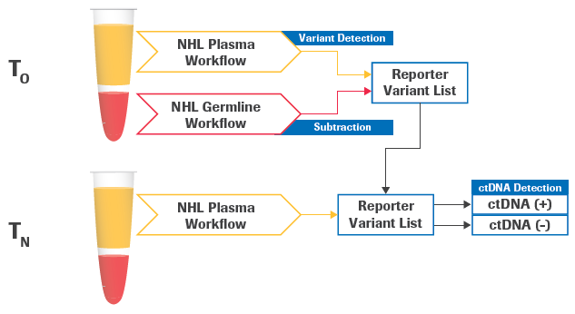
Figure 1. Schematic of longitudinal detection of circulating tumor DNA (ctDNA). The plasma and germline samples are obtained at a baseline time point T0. A new plasma sample is obtained at a follow-up time point TN to be evaluated for ctDNA detection. The analysis modules, from FASTQ processing to variant calling, can be applied to all three samples. Afterward, the longitudinal analysis module will utilize specific output files from the 3 samples, including BAM files and variant calls, to perform an evaluation of ctDNA detection at the follow-up timepoint. Image Credit: Roche Sequencing and Life Science
Note that where the text “SAMPLE” appears throughout the examples shown here, the user should replace it with a unique sample name. Similarly, replace “DESIGN” with the name of the target enrichment design that matches the design files supplied by Roche. “NumProcessors” should be replaced with the number of CPU cores available.
Users need to substitute “/path/to/...” in the provided examples with an appropriate path on their system. It is assumed that the current directory contains all input files, and it will also serve as the location for output files and report files.
This article discusses tools that necessitate running a .jar file via Java. An exception is the Genome Analysis Toolkit (GATK), which, while requiring Java, operates through a wrapper. Users whose default system version is not Java 1.8 must run the GATK .jar file by specifying a direct path to Java 1.8.
Despite how it may appear in the printed format, the entire command for each step should be entered on a single line. Ensure that there are no spaces within a file path. However, it is important to include spaces before and after each option in the command.
The backslash “\” at the end of a line is used for line continuation, usually for a long command. There should be no spaces after the backslash.
Due to idiosyncrasies in most—if not all—PDF viewers, the underscores in command line examples in this article may not display properly at all zoom percentages. One way to confirm whether or not underscores are present is to print the page. Alternatively, users could try temporarily switching to a very high zoom percentage (e.g., 400%).
Examples included in this article show how to perform the analysis with paired end Illumina sequencing reads. Many of the tools work with single end reads if paired end reads are not available, though input and output formats may vary.
Note that using single end reads will artificially increase the duplicate rate due to the decreased ability to resolve a unique fragment from the library.
Table 1. Third-party data analysis tools were used in this white paper. The examples described in this document were tested using the software versions listed in parentheses, and different software versions may require different function calls and/or flags. See section Reference Links for installation instructions and explanations of command options. These tools were tested on a Redhat Linux system. Many GATK4 tools were originally developed as part of Picard, which maintains detailed documentation referenced throughout this white paper. Source: Roche Sequencing and Life Science
| Package (version) |
Tool |
Function as used in this document |
| BWA (0.7.17) |
index |
Generate an indexed genome from FASTA sequence. |
| mem |
Map sequencing reads to an indexed genome. |
| FastQC (0.11.9) |
Fastqc |
Assess sequencing read quality (per-base quality plot). |
| GATK4* (4.2.0.0) |
BedToIntervalList |
Convert BED file to Genomic Interval List format. |
| CollectHsMetrics |
Assess performance of a target enrichment experiment based on mapped reads. |
| CollectAlignmentSummaryMetrics |
Report mapping metrics for a BAM file. |
| CollectInsertSizeMetrics |
Estimate and plot insert size distribution. |
| CountReads |
Count the number of sequencing reads overlapping target regions. |
| CreateSequenceDictionary |
Generate a sequence dictionary (.dict) for the reference genome. |
| FastqToSam |
Converts a FASTQ file to an unaligned BAM or SAM file. |
| IndexFeatureFile |
Generate an index (.idx) for a VCF file. |
| MarkDuplicates |
Count the number of optical duplicates. |
| MergeBamAlignment |
Merge alignment data from a SAM or BAM with data in an unmapped BAM file. |
| SamToFastq |
Convert a SAM or BAM file to a FASTQ file. |
| Java (>1.8.0_282) |
java |
Required for GATK4. |
| SAMtools (1.13) |
faidx |
Generate a FASTA index of the reference genome. |
| fastq |
Convert a BAM into FASTQ format. |
| flagstat |
Count the number of alignments for each FLAG type in a BAM file. |
| index |
Generate an index of the BAM file. |
| mpileup |
Generate text pileup output for the BAM file. |
| stats |
Produce comprehensive statistics from a BAM file. |
| sort |
Sort a BAM file. |
| view |
Select alignments based on the SAM FLAG value. |
| seqtk (1.3-r106) |
sample |
Randomly subsample FASTQ file(s). |
| fastp (0.20.1) |
fastp |
Trim raw reads for quality and sequenced primer/adapter. |
| fgbio (1.3.0) |
ExtractUmisFromBam |
Extract UMIs and store them in the RX tag of the BAM file. |
| GroupReadsByUmi |
Identify and group reads originating from the same source molecule. |
| CallMolecularConsensusReads |
Calculate the consensus sequence for each group of reads identified as originating from the same unique source molecule. |
| ClipBam |
Clipping overlapping reads in read pairs. |
| VarDict java (1.8.3) |
vardict-java |
Call somatic variants from a BAM file. |
| teststrandbias.R |
Perform a statistical test to detect strand bias. |
| var2vcf_valid.pl |
Convert the variant output from the intermediate tabular file into a VCF file. |
| BEDTools (2.30.0) |
intersect |
Screen for overlaps between two sets of genomic features. |
| SnpSift (4.3t) |
annotate |
Annotate variants with genomic database. |
| ctDNAtools (0.4.0) |
test_ctDNA |
Longitudinal mutation test. |
| create_background_panel |
Create background panel for longitudinal analysis. |
| create_black_list |
Create blocklist for longitudinal analysis. |
| get_background_rate |
Counts the base mismatches across target regions.
Divides sum of mismatches/sum of depths for all bases to get mismatch error rate. |
Reference genome and annotation
Before beginning the analysis, it is essential to select the appropriate human reference genome. The Longitudinal Mutation Analysis module employs the ctDNAtools package, 1 which necessitates installing a compatible BSgenome package from Bioconductor.
The BAM alignment files inputted into ctDNAtools must align with a reference genome supported by BSgenome, like BSgenome.Hsapiens.UCSC.hg38, to ensure optimal compatibility.
The complete list of genomes that BSgenome supports can be accessed by using the “available.genomes() function” in R.
More information on BSgenome can be found at https://bioconductor.org/packages/BSgenome. Examples of available human genomes include BSgenome.Hsapiens.UCSC.hg38, BSgenome.Hsapiens.NCBI.GRCh38, BSgenome.Hsapiens.UCSC.hg19, and BSgenome.Hsapiens.1000genomes.hs37d5.
If there is a preference for using a version of the human reference genome that is not supported by BSgenome, necessary alterations must be made within the scripts of the ctDNAtools package to achieve compatibility. Alternatively, creating a custom BSgenome data package is also a viable option.
The corresponding Database of Single Nucleotide Polymorphisms (dbSNP0) annotation database (Variant Call Format) .VCF file for the human reference genome can be obtained from NCBI dbSNP Builds (https://www.ncbi.nlm.nih.gov/snp/).
The hg38 dbSNP build 138 .VCF file is also available in the GATK resource bundle (https://console.cloud.google.com/storage/browser/genomics-public-data/resources/broad/ hg38/v0), which is described at https://gatk.broadinstitute.org/hc/en-us/articles/360035890811-Resource-bundle.
The dbSNP annotation is used to identify common Single Nucleotide Polymorphisms (SNPs) in variant calls. During reporter variant selection in the longitudinal analysis module, the common SNP variants are removed.
Index a reference genome
Before mapping can occur in most next-generation sequencing (NGS) applications, an indexed genome must be created. While various algorithms operate differently, the majority employ the Burrows-Wheeler (BWA) algorithm, which is effective for mapping millions of relatively short reads against the reference genome.
A genomic index is used to quickly identify the mapping location. Genomic indexing is required only once per genome version. The genomic index files that are created can then be used for all subsequent mapping jobs against that genome assembly version.
KDM Communications Ltd. recommends the FASTA formatted genome sequence be indexed with chromosomes in “karyotypic” sort order, i.e., chr1, chr2, ..., chr10, chr11, … chrX, chrY, chrM, etc. In these examples, reference genome files are referred to as “ref.fa”, which should be replaced by the actual file name (e.g., “hg38.fa”).
| Package⇨Tool(s) Used |
BWA⇨index
SAMtools⇨faidx
GATK⇨CreateSequenceDictionary |
| Input(s) |
ref.fa |
| Output(s) |
ref.fa {indexed}
- ref.fa = unmodified reference genome
- ref.fa.amb, ref.fa.ann, ref.fa.bwt, ref.fa.pac, ref.fa.sa = reference genome index files
- ref.fa.fai = FASTA index
- ref.dict = reference sequence dictionary
|
Generate Reference Genome Index
/path/to/bwa index -a bwtsw /path/to/ref.fa
Generate FASTA Index
/path/to/samtools faidx /path/to/ref.fa
Generate Sequence Dictionary
/path/to/gatk CreateSequenceDictionary --REFERENCE /path/to/ref.fa |
The use of an indexed reference genome in a later step is indicated by “ref.fa {indexed}” in the Input(s) section. An indexed reference genome includes the FASTA file of the genome along with all of its index files, which must be located in the same directory.
Note that multiple versions of the same reference genome can be available; thus, the user should select the appropriate genome for their analyses. It is essential for the user to confirm that the reference genome build used to create panel design files, such as primary target or capture target BED files, is identical to the one used in the analysis pipeline.
It is important to ensure that chromosome names are consistent between the two files in use. If the chosen version of the reference genome includes additional chromosomes or contigs (such as ALT contigs in the human reference), users must evaluate whether these elements are relevant and necessary for their specific analysis.
Certain areas of the human reference genome, like the pseudo-autosomal regions, can be depicted in various ways. These representations can significantly impact downstream analyses, including those related to variant analysis.
Decompress a FASTQ file
If the FASTQ files have been compressed (with a .GZ extension), some tools require them to be decompressed before use.
| Package⇨Tool(s) Used |
gunzip |
| Input(s) |
SAMPLE_R1.fastq.gz
SAMPLE_R2.fastq.gz |
| Output(s) |
SAMPLE_R1.fastq
SAMPLE_R2.fastq |
gunzip -c SAMPLE_R1.fastq.gz > SAMPLE_R1.fastq
gunzip -c SAMPLE_R2.fastq.gz > SAMPLE_R2.fastq |
Examine sequence read quality
Before spending time evaluating mapping statistics, use FASTQ on raw reads and generate a per-base sequence quality plot and report to evaluate sequencing quality. The FASTQ tool can work on both compressed and uncompressed FASTQ files.
| Package⇨Tool(s) Used |
FastQC⇨fastqc |
| Input(s) |
SAMPLE_R1.fastq / SAMPLE_R1.fastq.gz
SAMPLE_R2.fastq / SAMPLE_R2.fastq.gz |
| Output(s) |
SAMPLE_R1_fastqc.zip
SAMPLE_R2_fastqc.zip |
| /path/to/fastqc --nogroup --extract SAMPLE_R1.fastq(.gz) SAMPLE_R2.fastq(.gz) |
FastQC has a --threads option that allows users to specify the number of files that can be processed simultaneously. FastQC describes, “Each thread will be allocated 250MB of memory so the user shouldn’t run more threads than their available memory will cope with, and not more than 6 threads on a 32 bit machine”.
In the provided example, users have the option to use the --threads 2 command to accelerate the calculation process. For each SAMPLE input file, a .zip file is generated. Additionally, an HTML report named fastqc_report.html is created, which can be viewed using an internet browser.
The authors of FastQC have posted the following examples of the Quality Control (QC) report for a good and a bad sequencing run:
http://www.bioinformatics.babraham.ac.uk/projects/fastqc/good_sequence_short_fastqc.html
http://www.bioinformatics.babraham.ac.uk/projects/fastqc/bad_sequence_fastqc.html
Remove duplicates by utilizing unique molecular identifiers (UMIs)
The recommended methodology to obtain consensus reads from Polymerase Chain Reaction (PCR) and optical duplicates are described in this section. It is specific to sequencing data from libraries constructed using the KAPA Universal Unique Molecular Identifiers (UMIs) Adapter and the KAPA Unique Device Identification (UDI) Primer Mixes.
The methodology illustrated below consists of three steps:
1) Extraction of the UMI from insert reads;
2) Grouping of these UMIs into families/groups based on alignment coordinates and UMI sequence composition; and
3) Consensus calling of all reads within a particular UMI group.
The Roche UMI adapters described above utilize a mix of “fixed” sequence adapters. In case the exact UMI sequences are needed for additional analysis, refer to Table 2 on the following page.
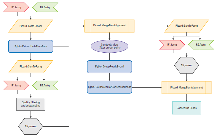
Figure 2. Recommended pipeline for UMI extraction, grouping, and consensus read calling. Image Credit: Roche Sequencing and Life Science
Table 2. Sequence mix of the Roche UMI adapters (KAPA Universal UMI Adapter) The bolded T is the 3' T-overhang of the adapter. The sequence in italics is not part of the UMI sequence; it is added to increase the sequence diversity in order to ensure optimal sequencing performance. Source: Roche Sequencing and Life Science
| UMI family |
Sequence |
| 1 |
AATCCT |
| 2 |
AGAAGT |
| 3 |
CCAGGT |
| 4 |
CTTACT |
| 5 |
GAAGCT |
| 6 |
GGTCGT |
| 7 |
TCTAGT |
| 8 |
TTACCT |
| 9 |
ACCT |
| 10 |
ATGT |
| 11 |
CAGT |
| 12 |
CGCT |
| 13 |
GCGT |
| 14 |
GTCT |
| 15 |
TACT |
| 16 |
TGGT |
Convert FASTQ to binary alignment/map (BAM)
The first step is to convert the demultiplexed, raw-sequencing FASTQ files to BAM files using the FastqToSam tool in GATK.
| Package⇨Tool(s) Used |
GATK⇨FastqToSam |
| Input(s) |
SAMPLE_R1.fastq.gz
SAMPLE_R2.fastq.gz |
| Output(s) |
SAMPLE_unmapped.bam |
| /path/to/gatk FastqToSam \
-F1 SAMPLE_R1.fastq.gz \
-F2 SAMPLE_R2.fastq.gz \
-O SAMPLE_unmapped.bam \
-SM SAMPLE
|
Extract UMIs from BAM
The read structure is specified as 3M3S+T. This involves extracting the first three bases, which are then stored as the UMI in the RX tag of the BAM file, as indicated by the 3M component of the structure.
Remove the next three bases from the beginning of the read (indicated as 3S). These bases form a punctuation sequence, which is used to enhance the sequence diversity and thereby ensure optimal sequencing performance.
Maintain the remaining sequence as part of the insert read (+T). The UMIs extracted from read 1 and read 2 are stored in the RX tag of the unmapped BAM file as UMI1-UMI2 (hereafter referred to as “the UMI” and considered as a single sequence).
| Package⇨Tool(s) Used |
fgbio⇨ExtractUmisFromBam |
| Input(s) |
SAMPLE_unmapped.bam |
| Output(s) |
SAMPLE_unmapped_umi_extracted.bam |
| /path/to/fgbio ExtractUmisFromBam \
-i SAMPLE_unmapped.bam \
-o SAMPLE_unmapped_umi_extracted.bam \
-r 3M3S+T 3M3S+T \
-t RX \
-a true
|
Perform adapter trimming and quality filtering
The BAM file containing reads with extracted UMIs must be converted to a FASTQ format to facilitate adapter trimming and quality filtering. It is important to perform adapter trimming and quality filtering only after UMI extraction. This approach prevents potential bias and guarantees that only the template or insert is trimmed.
In this workflow, the unmapped BAM file is initially converted to a FASTQ file using GATK. Following this, adapter trimming and quality filtering are executed with fastp. The parameters are configured to allow automatic detection of adapter sequences, or users can manually set adapter sequences, as detailed in the Illumina Adapter Sequences Document #1000000002694 v.11 or later versions.
Note: Converting BAM files to FASTQ format does not preserve the extracted UMI information. Therefore, it is crucial to keep the output file from the UMI extraction process, named SAMPLE_unmapped_umi_extracted.bam. This file retains the UMI data stored in the RX tag, which is essential for subsequent processes after genomic alignment.
| Package⇨Tool(s) Used |
GATK⇨SamToFastq
fastp |
| Input(s) |
SAMPLE_unmapped_umi_extracted.bam |
| Output(s) |
SAMPLE_umi_extracted_trimmed_R1.fastq
SAMPLE_umi_extracted_trimmed_R2.fastq
SAMPLE_fastp.log |
Convert BAM to FASTQ
/path/to/gatk SamToFastq \
-I SAMPLE_unmapped_umi_extracted.bam \
-F SAMPLE_umi_extracted_R1.fastq \
-F2 SAMPLE_umi_extracted_R2.fastq \
--CLIPPING_ATTRIBUTE XT \
--CLIPPING_ACTION 2
Perform Adapter and Quality Trimming
/path/to/fastp \
-i SAMPLE_umi_extracted_R1.fastq \
-o SAMPLE_umi_extracted_trimmed_R1.fastq \
-I SAMPLE_umi_extracted_R2.fastq \
-O SAMPLE_umi_extracted_trimmed_R2.fastq \
-g -W 5 -q 20 -u 40 -x -3 -l 75 -c \
-j fastp.json \
-h fastp.html \
-w NumProcessors &> SAMPLE_fastp.log
|
The -3 and -W 5 options allow trimming from the 3’ tail in a sliding window of 5 bp. If the mean quality is below the quality set by -q, the bases are trimmed. In addition, -u specifies what percent of bases are allowed to be unqualified before a read is discarded.
The -x and -g options turn on poly X and poly G tail trimming, respectively. The -l option means the length of the trimmed read must be at least 50 bp. The -c option turns on base correction for read pairs where read1 and read2 overlap.
The fastp application will produce two files. The SAMPLE_umi_extracted_trimmed_R1.fastq and SAMPLE_umi_extracted_ trimmed_R2.fastq contain the reads that are still paired after adapter trimming and quality filtering.
Unpaired reads can optionally be assigned to output files using the --unpaired1 and --unpaired2 options. If the user wants to increase the percentage of passing reads, the quality and length filter thresholds can be lowered.
Select a subsample of reads from a FASTQ file
Random subsampling is useful for normalizing the number of reads per set when making comparisons. With paired end reads, it is important that the two files use the same values for the seed (-s) and number of reads. The seqtk application can write the sampled reads to uncompressed FASTQ files.
| Package⇨Tool(s) Used |
seqtk⇨sample |
| Input(s) |
SAMPLE_umi_extracted_trimmed_R1.fastq
SAMPLE_umi_extracted_trimmed_R2.fastq |
| Output(s) |
SAMPLE_umi_extracted_trimmed_subset_R1.fastq
SAMPLE_umi_extracted_trimmed_subset_R2.fastq |
/path/to/seqtk sample -s 12345 SAMPLE_umi_extracted_trimmed_R1.fastq 40000000 > SAMPLE_umi_extracted_trimmed_subset_R1.fastq
/path/to/seqtk sample -s 12345 SAMPLE_umi_extracted_trimmed_R2.fastq 40000000 > SAMPLE_umi_extracted_trimmed_subset_R2.fastq |
The commands above will randomly subsample 40 million matched read pairs from the paired end FASTQ files for a total of 80 million reads per sample. Supplying the same random seed value (-s) ensures that the FASTQ records will remain in synchronized sort order and can be used for mapping, etc.
Note that seqtk requires an amount of Random Access Memory (RAM) proportional to the number of reads being subsampled. As the user increases the size of the subsampled read set, more RAM is needed.
Map reads to the reference genome
Adapter trimmed and quality-filtered reads are mapped to the indexed reference genome using BWA.
| Package⇨Tool(s) Used |
BWA⇨mem |
| Input(s) |
SAMPLE_umi_extracted_trimmed_R1.fastq (shown below) or
SAMPLE_umi_extracted_trimmed_subset_R1.fastq if subsampling
SAMPLE_umi_extracted_trimmed_R2.fastq (shown below) or
SAMPLE_umi_extracted_trimmed_subset_R2.fastq if subsampling
ref.fa {indexed} |
| Output(s) |
SAMPLE_umi_aligned.bam |
| /path/to/bwa mem \
-R “@RG\\tID:A\\tDS:KAPA_TE\\tPL:ILLUMINA\\tLB:SAMPLE\\tSM:SAMPLE” \
-t NumProcessors \
-Y \
/path/to/ref.fa \
SAMPLE_umi_extracted_trimmed_R1.fastq \
SAMPLE_umi_extracted_trimmed_R2.fastq \
| \
samtools view -f2 -Sb > SAMPLE_umi_aligned.bam |
In the “Map Reads” step, the -R option defines the read group (“@RG”), which will appear in the BAM header. Within this string is the sample ID (“ID”), description field (“DS”), sequencing platform (“PL”), library name (“LB”), and sample name (“SM”). When a library name, ID, and sample name do not separately exist, a SAMPLE descriptor may be used, as shown in the example above.
The -Y option uses soft clipping for supplementary alignments. It is advisable to keep only reads that are aligned in proper pairs in BAM. The tool samtools_view and the flag -f2 can be used for this purpose.
Add UMI information to the reads in BAM
As UMI information is not retained during BAM to FASTQ conversion, it is necessary to merge the two BAM files containing the UMI information (SAMPLE_unmapped_umi_extracted.bam) and the alignment coordinate information (SAMPLE_ umi_aligned.bam).
The UMI information is now stored in the RX tag of the new umi_extracted_aligned_merged.bam file. MergeBamAlignment requires queryname sorted inputs.
| Package⇨Tool(s) Used |
GATK⇨SortSam
GATK⇨MergeBamAlignment |
| Input(s) |
SAMPLE_umi_aligned.bam
SAMPLE_unmapped_umi_extracted.bam
ref.fa {indexed} |
| Output(s) |
SAMPLE_umi_extracted_aligned_merged.bam |
/path/to/gatk SortSam \
--I=SAMPLE_umi_aligned.bam \
--O=SAMPLE_umi_aligned_qnsorted.bam \
--SORT_ORDER=”queryname”
/path/to/gatk MergeBamAlignment \
--ATTRIBUTES_TO_RETAIN X0 \
--ATTRIBUTES_TO_REMOVE NM \
--ATTRIBUTES_TO_REMOVE MD \
--ALIGNED_BAM SAMPLE_umi_aligned_qnsorted.bam \
--UNMAPPED_BAM SAMPLE_unmapped_umi_extracted.bam \
--OUTPUT SAMPLE_umi_extracted_aligned_merged.bam \
--REFERENCE_SEQUENCE /path/to/ref.fa \
--SORT_ORDER queryname \
--ALIGNED_READS_ONLY true \
--MAX_INSERTIONS_OR_DELETIONS -1 \
--PRIMARY_ALIGNMENT_STRATEGY MostDistant \
--ALIGNER_PROPER_PAIR_FLAGS true \
--CLIP_OVERLAPPING_READS false |
Identify and group reads originating from the same source molecule
The GroupReadsByUmi tool in fgbio utilizes the UMI (UMI1-UMI2) and the genomic alignment start site to assign unique source molecules to each applicable read. GroupReadsByUmi implements the adjacency strategy introduced by UMI- tools.
The user can control how many errors/mismatches are allowed in the UMI sequence when assigning source molecules (--edits=n). UMI group statistics are output to a SAMPLE_umi_group_data.tsv file using the -f flag.
Note: The parameter --edits=1 will account for a single mismatch in the entire UMI sequence (UMI1+UMI2). Altering this parameter to >1 will have a significant impact on the outcome of the UMI grouping algorithm and the resultant UMI groups.
| Package⇨Tool(s) Used |
fgbio⇨GroupReadsByUmi |
| Input(s) |
SAMPLE_umi_extracted_aligned_merged_filtered.bam |
| Output(s) |
SAMPLE_umi_grouped.bam
SAMPLE_umi_group_data.tsv |
/path/to/fgbio GroupReadsByUmi \
--input=SAMPLE_umi_extracted_aligned_merged_filtered.bam \
--output=SAMPLE_umi_grouped.bam \
--strategy=adjacency \
--edits=1 \
-t RX \
-f SAMPLE_umi_group_data.tsv |
Calculate consensus sequence
The CallMolecularConsensusReads tool in fgbio processes each group of reads identified as originating from the same unique source molecule. The consensus of a group of reads can only be calculated if there are a minimum of two reads in a group.
Reads that occur as singletons are discarded by default, but this can be changed by setting the –min-reads flag to 1, and the single read will be considered the consensus.
Note: Bases with a sequencing quality less than 20 will not be used in the consensus calculation, but this can also be altered with the –min-input-base-quality flag.
Note: Here, reads are defined as those grouped into a UMI family/group, i.e., reads that have the same UMI tag and the same 5’ start position. Furthermore, the two reads minimum could consist of two reads from the same unique source molecule, or one read derived from the forward template of the unique source molecule and one derived from the reverse template of the unique source molecule.
| Package⇨Tool(s) Used |
fgbio⇨CallMolecularConsensusReads |
| Input(s) |
SAMPLE_umi_grouped.bam |
| Output(s) |
SAMPLE_umi_consensus_unmapped.bam |
/path/to/fgbio CallMolecularConsensusReads \
--input=SAMPLE_umi_grouped.tsorted.bam \
--output=SAMPLE_umi_consensus_unmapped.bam \
--error-rate-post-umi 40 \
--error-rate-pre-umi 45 \
--output-per-base-tags false \
--min-reads 1 \
--max-reads 100 \
--min-input-base-quality 20 \
--read-name-prefix=’consensus’ |
Filter consensus reads
The FilterConsensusReads tool in fgbio is used to filter consensus reads generated by CallMolecularConsensusReads.
The option ––max-read-error-rate is the maximum raw-read error rate across the entire consensus read. The option ––max–base–error–rate is the maximum error rate for a single consensus base. The option ––max–no–call–fraction is the maximum fraction of no-calls in the read after filtering.
The option ––min– base–quality is the minimum mean base quality across the consensus read. The option ––min–reads is the minimum number of reads supporting a consensus read. The option ––reverse–per–base–tags controls whether per-base tags should be reversed before being used on reads marked as being mapped to the negative strand.
| Package⇨Tool(s) Used |
fgbio⇨FilterConsensusReads |
| Input(s) |
SAMPLE_umi_consensus_unmapped.bam
ref.fa {indexed} |
| Output(s) |
SAMPLE_umi_consensus_unmapped_filtered.bam |
/path/to/fgbio FilterConsensusReads \
--input=SAMPLE_umi_consensus_unmapped.bam \
--output=SAMPLE_umi_consensus_unmapped_filtered.bam \
--ref=/path/to/ref.fa \
--max-read-error-rate=0.025 \
--max-base-error-rate=0.1 \
--max-no-call-fraction=0.1 \
--min-base-quality=20 \
--min-reads=1 \
--reverse-per-base-tags=true |
Convert BAM to FASTQ
After consensus calling, the collapsing of the UMI groups results in the loss of alignment coordinate information. To rectify this, the SAMPLE_umi_consensus_unmapped.bam is converted to FASTQ format using SamToFastq in GATK.
Note: Loss of alignment coordinates is an inherent limitation of consensus calling and is related to alignment quality. When base information is statistically extrapolated from two or more molecules, the alignment quality is also statistically averaged. Many downstream variant callers rely on alignment quality; thus, to avoid error, the consensus reads are realigned to ensure correct alignment qualities.
| Package⇨Tool(s) Used |
GATK⇨SortSam
GATK⇨SamToFastq |
| Input(s) |
SAMPLE_umi_consensus_unmapped_filtered.bam |
| Output(s) |
SAMPLE_umi_consensus_unmapped_R1.fastq
SAMPLE_umi_consensus_unmapped_R2.fastq |
/path/to/gatk SortSam \
I=SAMPLE_umi_consensus_unmapped_filtered.bam \
O=SAMPLE_umi_consensus_unmapped_filtered_qnsorted.bam \
SORT_ORDER=”queryname”
/path/to/gatk SamToFastq \
-I SAMPLE_umi_consensus_unmapped_filtered_qnsorted.bam \
-F SAMPLE_umi_consensus_unmapped_R1.fastq \
-F2 SAMPLE_umi_consensus_unmapped_R2.fastq \
--CLIPPING_ATTRIBUTE XT \
--CLIPPING_ACTION 2 |
Map consensus reads to the reference genome
A new SAMPLE_umi_consensus_mapped.bam file is generated after aligning the consensus reads to the indexed reference genome using BWA.
| Package⇨Tool(s) |
Used BWA⇨mem |
| Input(s) |
SAMPLE_umi_consensus_unmapped_R1.fastq
SAMPLE_umi_consensus_unmapped_R2.fastq
ref.fa {indexed} |
| Output(s) |
SAMPLE_umi_consensus_mapped.bam |
/path/to/bwa mem \
-R “@RG\\tID:A\\tDS:KAPA_TE\\tPL:ILLUMINA\\tLB:SAMPLE\\tSM:SAMPLE” \
-Y \
-t NumProcessors \
/path/to/ref.fa \
SAMPLE_umi_consensus_unmapped_R1.fastq \
SAMPLE_umi_consensus_unmapped_R2.fastq \
l \
samtools view -bh - > SAMPLE_umi_consensus_mapped.bam |
Add UMI information to the consensus reads in BAM
The final step is to merge the SAMPLE_umi_consensus_mapped.bam with the SAMPLE_umi_consensus_unmapped.bam to retain the UMI group information. This will yield an aligned BAM file with consensus reads and the UMI information retained in the RX flag. The BAM file will be coordinated and sorted, and a .bai index file will be produced.
| Package⇨Tool(s) Used |
GATK⇨SortSam
GATK⇨MergeBamAlignment |
| Input(s) |
SAMPLE_umi_consensus_mapped.bam
SAMPLE_umi_consensus_unmapped.bam
ref.fa {indexed} |
| Output(s) |
SAMPLE_umi_deduped.bam |
/path/to/gatk SortSam \
I=SAMPLE_umi_consensus_mapped.bam \
O=SAMPLE_umi_consensus_mapped_qnsorted.bam \
SORT_ORDER=”queryname”
/path/to/gatk MergeBamAlignment \
--ATTRIBUTES_TO_RETAIN X0 \
--ATTRIBUTES_TO_RETAIN RX \
--ALIGNED_BAM SAMPLE_umi_consensus_mapped_qnsorted.bam \
--UNMAPPED_BAM SAMPLE_umi_consensus_unmapped_filtered_qnsorted.bam \
--OUTPUT SAMPLE_umi_deduped_sorted.bam \
--REFERENCE_SEQUENCE /path/to/ref.fa \
--SORT_ORDER coordinate \
--ADD_MATE_CIGAR true \
--MAX_INSERTIONS_OR_DELETIONS -1 \
--PRIMARY_ALIGNMENT_STRATEGY MostDistant \
--ALIGNER_PROPER_PAIR_FLAGS true \
--CLIP_OVERLAPPING_READS false \
--ADD_PG_TAG_TO_READS false \
--UNMAPPED_READ_STRATEGY COPY_TO_TAG \
--ORIENTATIONS FR \
--CREATE_INDEX true |
Clip overhangs
Read overhangs can be clipped using the fgbio ClipBam tool to avoid double counting variant-supporting reads from the same template. This is recommended prior to variant calling.
| Package⇨Tool(s) Used |
gatk⇨SortSam
fgbio⇨ClipBam |
| Input(s) |
SAMPLE_umi_deduped_sorted.bam |
| Output(s) |
SAMPLE_umi_deduped_qnsorterd_clipov.bam
SAMPLE_clipov_metrics.txt |
/path/to/gatk SortSam \
I=SAMPLE_umi_deduped_sorted.bam \
O=SAMPLE_umi_deduped_qnsorted.bam \
SORT_ORDER=”queryname”
/path/to/fgbio ClipBam \
--clip-overlapping-reads \
-i SAMPLE_umi_deduped_qnsorted.bam \
-o SAMPLE_umi_deduped_qnsorterd_clipov.bam \
-m SAMPLE_clipov_metrics.txt \
-r path/to/ref.fa |
Sort BAM and create index
The BAM files need to be sorted and indexed for use in the subsequent steps. Here, the indices for the BAM files are sorted and created both before and after the UMI deduplication. The BAM files can now be used for all downstream applications and analyses described by the particular NGS analysis workflow.
| Package⇨Tool(s) Used |
gatk⇨SortSam |
| Input(s) |
SAMPLE_umi_aligned.bam
SAMPLE_umi_deduped.bam |
| Output(s) |
SAMPLE_umi_aligned_sorted.bam
SAMPLE_umi_aligned_sorted.bai
SAMPLE_umi_deduped_clipov_sorted.bam
SAMPLE_umi_deduped_clipov_sorted.bai |
Sort and Index the Non-deduped BAM
/path/to/gatk SortSam \
I=SAMPLE_umi_aligned.bam \
O=SAMPLE_umi_aligned_sorted.bam \
SORT_ORDER=”coordinate” \
CREATE_INDEX=true
Sort and Index the UMI Deduped Overhang-Clipped BAM
/path/to/gatk SortSam \
I=SAMPLE_umi_deduped_qnsorterd_clipov.bam \
O=SAMPLE_umi_deduped_clipov_sorted.bam \
SORT_ORDER=”coordinate” \
CREATE_INDEX=true |
Detect single nucleotide variant (SNV) in baseline sample
After reads are mapped, and duplicates are removed, variants are often called against the reference genome. Somatic variants must be called by callers that are capable of detecting low abundance variants. This next section will outline how to use VarDict to call somatic variants.
VarDict is a widely recognized somatic caller, renowned for its ultra-sensitivity in detecting variants from targeted sequencing data. VarDict’s performance scales linearly to sequencing depth, and it enables ultra-deep sequencing for tumor evolution and liquid biopsy.
Originally written in Perl as vardict.pl, the tool has been developed with a Java-based replacement, which yields ten times more acceleration than the Perl implementation. For longitudinal analysis, the set of SNVs detected in the baseline sample will be used as reporter variant candidates for analysis.
| Package⇨Tool(s) Used |
vardict-java
teststrandbias.R
var2vcf_valid.pl |
| Input(s) |
ref.fa {indexed}
SAMPLE_umi_deduped_clipov_sorted.bam
DESIGN_capture_targets.bed |
| Output(s) |
SAMPLE_vardict.vcf |
/path/to/vardict-java \
-G /path/to/ref.fa \
-f 0.005 \
-N SAMPLE \
-b SAMPLE_umi_deduped_clipov_sorted.bam \
-c 1 -S 2 -E 3 -g 4 DESIGN_capture_targets.bed l \
/path/to/teststrandbias.R l \
/path/to/var2vcf_valid.pl -N SAMPLE -E -f 0.005 > SAMPLE_vardict.vcf |
Annotate variants
The variants can be annotated with dbSNP using the SnpSift tool. The dbSNP annotation is used in the longitudinal analysis module to remove common SNPs.
| Package⇨Tool(s) Used |
SnpSift⇨annotate |
| Input(s) |
SAMPLE_vardict.vcf
dbsnp.vcf.gz |
| Output(s) |
SAMPLE_vardict_annotated.vcf |
/path/to/SnpSift annotate \
-name “DBSNP_” \
-info CAF,COMMON \
/path/to/dbsnp.vcf.gz > SAMPLE_vardict_annotated.vcf |
VCF to table
The annotated VCF file can be parsed into a tab-delimited table for downstream processing using GATK VariantsToTable. VCF standard and INFO fields can be extracted using the option -F. The genotype FORMAT fields can be extracted using the option -GF.
The output text file is used for downstream longitudinal analysis. The recommended fields to extract from the vardict VCF file should include the following: AF: Allele frequency; DP: Depth – total depth; VD: AltDepth – variant depth; MQ: mapping quality; QUAL: average base quality at a variant position; SBF: Strand Bias Fisher p-value; NM: mean mismatches in reads.
These fields are used for filtering during the reporter variant selection step in longitudinal mutation analysis.
| Package⇨Tool(s) Used |
gatk⇨VariantsToTable |
| Input(s) |
SAMPLE_vardict_annotated.vcf |
| Output(s) |
SAMPLE_vardict_annotated_vcf.txt |
/path/to/gatk VariantsToTable \
-V SAMPLE_vardict_annotated.vcf \
--show-filtered \
-F CHROM -F POS -F REF -F ALT -F ID -F FILTER \
-F ADJAF -F AF -F BIAS -F DP -F VD -F DUPRATE \
-F END -F HIAF -F MQ -F HICNT -F HICOV -F LSEQ \
-F RSEQ -F NM -F PSTD -F QSTD -F QUAL -F REFBIAS \
-F VARBIAS -F SBF -F SN -F TYPE \
-F DP4 -F HRUN -F SB -F DBSNP_CAF -F DBSNP_COMMON \
-GF AD -GF ALD -GF GT -GF RD \
-O SAMPLE_vardict_annotated_vcf.txt |
Longitudinal mutation analysis
Description
Longitudinal mutation analysis involves using a set of reporter variants detected in a baseline cell-free DNA (cfDNA) sample to track and detect the same variants in subsequent follow-up cfDNA sample(s).
Detection in the follow-up sample is based on the number of variant-supporting reads observed. A mutation-positive follow-up sample would have variant-supporting reads that are significantly higher than the background error rate.
An empirical p-value from a Monte-Carlo sampling-based test is used for mutation positivity calling, based on the approach by Newman et al.2 The ctDNAtools package provides tools to implement the longitudinal mutation analysis. The main components included in the analysis are 1) Generate background panel and blocklist, 2) Select reporter variants, and 3) Evaluate longitudinal mutations.
Three different samples are used for the longitudinal analysis. The reporter variants are obtained from the baseline cfDNA sample. The germline sample is used to remove reporters observed in the germline.
The follow-up sample is tested for mutation positivity based on the reporter variants. If multiple follow-up samples are subsequently obtained, the analysis can be performed using the same respective baseline and germline samples.
In addition, a set of normal cfDNA samples is required to generate a longitudinal analysis blocklist, which is used to establish a list of error-prone mutations in the panel target regions.
A list of R packages required by ctDNAtools can be found at https://github.com/alkodsi/ctDNAtools/blob/master/DESCRIPTION.
Importantly, the appropriate BSgenome.Hsapiens library needs to be used. (See previous section “Reference Genome and Annotation”).
In addition, the R package, optparse, is required for implementing the modules described in this article using custom scripts. All of the custom scripts described here in the longitudinal analysis can be obtained from https://github. com/Roche-CSI/kapa_nhl. This table summarizes the R packages required:
R (≥3.6.0)
magrittr
dplyr (≥0.8.3)
tidyr (≥1.0.0)
purrr (≥0.3.2)
Rsamtools (≥2.0.0)
assertthat (≥0.2.1)
GenomicRanges
IRanges
GenomeInfoDb
BiocGenerics
BSgenome
GenomicAlignments
rlang (≥0.4.0)
Biostrings
methods
furrr (≥0.1.0)
ellipsis (≥0.3.0)
VariantAnnotation (≥1.30.1)
GenomeInfoDbData
optparse
BSgenome.Hsapiens (version according to genome choice) |
Generate background panel and blocklist
Longitudinal analysis involves the detection of minor amounts of variant-supporting reads, often below 0.1% allele frequency (AF). A blocklist is highly recommended to filter out variants that are likely to be false positives.
This section will discuss how to generate a blocklist using a set of normal samples with the ctDNAtools package in custom scripts.
The blocklist only needs to be generated once for the longitudinal workflow setup. After the blocklist is obtained, all subsequent analyses will be able to use the same blocklist.txt file. A new blocklist is recommended whenever there are major changes to the workflow, such as new reagents, capture probe panels, or protocols.
The create_bg_panel.R and the create_blocklist.R scripts will utilize the functions create_background_panel and create_black_list from ctDNAtools, respectively.
A background panel file is required prior to generating the blocklist. This is obtained using the create_bg_panel.R script. A .csv file without column headers that contain the path to the bam files from normal samples is used as input, as well as the target region bed file.
The output is a panel_background.RDS file that contains information such as read depth and alt AF for background mutations. The file can be read into the R environment using the function readRDS().
Two types of blocklists are available in the ctDNAtools package. The first type is a list of genomic loci (chr_pos, regardless of substitutions). The second type is substitution-specific (chr_pos_ref_alt), which offers a more specific variant-level list for identifying errors.
The blocklist type can be set using the option ––blist_type during the create_bg_panel.R process. Setting it to “loci” will implement a loci-based list, whereas setting it to “variant” will implement a substitution-specific list.
Lastly, the BSgenome.Hsapiens version should match the reference for the input sample bam files. For example, setting the option ––reference to “BSgenome.Hsapiens.UCSC.hg38” will load BSgenome.Hsapiens.UCSC.hg38.
After the panel_background.RDS file is obtained, the create_blocklist.R script can be used to generate the blocklist.txt file. The selection of parameters in the blocklist creation is critical to identify which loci are considered to be background noise.
The quantile of mean VAF above which the loci are considered noise is set using ––blocklist_ vaf_quantile. A blocklist should be built using a sufficient number of normal samples to capture the error-prone regions in the panel.
The minimum number of normal samples that exhibit at least one non-reference read to be considered noisy is set using ––blocklist_min_samples_one_read. The minimum number of normal samples that exhibit at least two non-reference reads to be considered noisy is set using ––blocklist_min_samples_two_reads.
The minimum number of normal samples that exhibit at least n non-reference reads is set using ––blocklist_min_samples_n_reads. It is recommended to set ––blocklist_min_samples_one_read at greater than 60% of the number of normal samples.
For example, if there are 20 normal samples used for generating the blocklist, ––blocklist_min_samples_one_read should be set to 12. This would allow error-prone variants to be captured efficiently when they occur in at least 12 normal samples.
Similarly, for ––blocklist_min_samples_two_reads, it is recommended to be set at greater than 50% of the number of normal samples. Parameters for blocklist generation should be experimentally determined to obtain optimal results.
| Package⇨Tool(s) Used |
create_bg_panel.R
create_blocklist.R
ctDNAtools ⇨ create_background_panel
ctDNAtools ⇨ create_black_list |
| Input(s) |
umi_deduped_sorted_bams.csv
(list of normal sample bam files) |
| Output(s) |
blocklist.txt
panel_background.RDS |
Create background panel
Rscript create_bg_panel.R \
--bam_list umi_deduped_sorted_bams.csv \
--panel_background panel_background.RDS \
--target_bed DESIGN_capture_targets.bed \
--blist_type variant \
--reference BSgenome.Hsapiens.UCSC.hg38
Create blocklist
Rscript create_blocklist.R \
--panel_background panel_background.RDS \
--blocklist blocklist.txt \
--vaf_quantile 0.95 \
--min_samples_one_read 12 \
--min_samples_two_reads 10 |
Select reporter variants
The list of reporter variant candidates after variant calling by vardict-java should be filtered to obtain confident reporters for longitudinal analysis. Filtering according to variant metrics is performed, followed by germline presence detection.
Only SNVs are used for longitudinal analysis. Reporter variant candidates that do not meet filtering criteria will be removed from downstream longitudinal analysis. The recommended filters for keeping high-confidence somatic SNV reporters are: FILTER=PASS, AF>0.5%, AF<35%, DP>1000, VD>15, MQ>55, QUAL>45.
In addition, variants included in the dbSNP database are removed. More stringent filtering may be applied to reduce the number of false reporter variants. These options are available in the filter_reporters.R script. The default filtering thresholds for the script are shown on the following page.
After variant filtering, the remaining reporter variant candidates are examined for germline sample presence. The germline sample bam file is set using the --germline option. If the same variant is detected in the germline sample, it is removed from downstream analysis.
The germline presence AF threshold can be set using the --germline_af option. A stringent cutoff, such as 0.0005, will remove reporter variant candidates that have detectable reads in the germline sample at 0.05% AF. Reporter candidates included in the blocklist.txt file will also be removed from downstream longitudinal analysis.
The final selected list of baseline reporter variants used for longitudinal analysis are saved in the output file selected_baseline_reporters.txt. To assist in the manual review process, all potential reporters will be annotated with corresponding germline sample data and follow-up sample read counts. This information will be compiled in the ‘all_reporters.txt’ file after the variant filtering step.
The reads to be included for counting can be filtered by ––read_min_bq (minimum base quality) and ––read_ min_mq (minimum mapping quality). The ––read_max_dp option is the maximum depth above which sampling will happen.
| Package⇨Tool(s) Used |
select_reporters.R |
| Input(s) |
BASELINE_SAMPLE_vardict_annotated.vcf.txt
GERMLINE_SAMPLE_umi_deduped.clipov.sorted.bam
FOLLOWUP_SAMPLE_umi_deduped.clipov.sorted.bam
blocklist.txt |
| Output(s) |
selected_baseline_reporters.txt
selected_baseline_reporters.vcf
all_reporters.txt |
Rscript select_reporters.R \
--filter_reporters TRUE \
--remove_snp TRUE \
--reporters BASELINE_SAMPLE_vardict_annotated_vcf.txt \
--germline GERMLINE_SAMPLE_umi_deduped_clipov_sorted.bam \
--followup FOLLOWUP_SAMPLE_umi_deduped_clipov_sorted.bam \
--selected selected_baseline_reporters.txt \
--selected_vcf selected_baseline_reporters.vcf \
--all all_reporters.txt \
--blocklist blocklist.txt \
--germline_cutoff 0.005 \
--min_af 0.005 \
--max_af 0.35 \
--min_dp 1000 \
--min_vd 15 \
--min_mq 55 \
--min_qual 45 \
--min_sbf 0.00001 \
--max_nm 4 \
--read_min_bq 30 \
--read_min_mq 30 \
--read_max_dp 20000 |
Evaluate longitudinal mutations
Finally, the set of selected reporters are used for evaluating longitudinal mutations and determining mutation positivity in the follow-up cfDNA sample. The longitudinal_analysis.R script will run the test_ctDNA function from ctDNAtools.
The reporters listed in the selected_baseline_reporters.txt file will be used to query the follow-up sample BAM file FOLLOWUP_SAMPLE_umi_deduped.clipov.sorted.bam to evaluate mutation positivity.
The primary steps are as follows:
- Quantifying the read counts for both reference and variant alleles of the reporter variants.
- Estimating the background rate of the tested sample.
- Utilizing a Monte Carlo-based sampling test to calculate an empirical p-value.
The p-value will only be used to determine positivity if the number of informative reads (number of all unique reads covering the mutations) exceeds the specified threshold. Otherwise, the sample will be considered undetermined.
The threshold for the number of informative reads is established through the ––reads_threshold option. The p-value threshold for determining ctDNA positivity or negativity is set using the ––pvalue_threshold option. To optimize sensitivity and specificity, it is important to carefully determine the appropriate p-value threshold.
A set of normal cfDNA samples can be used to test the range of p-values to call ctDNA negativity. When calculating the background rate, the ––vaf_threshold is used to ignore the bases with higher than the VAF threshold (likely true mutations).
The ––read_min_bq, ––read_min_mq, and ––read_max_dp are options used for read counting, which are the same options as the select_reporters.R script in the previous step. The ––n_sim option is the number of Monte Carlo simulations.
| Package⇨Tool(s) Used |
longitudinal_analysis.R
ctDNAtools ⇨ test_ctDNA |
| Input(s) |
selected_baseline_reporters.txt
FOLLOWUP_SAMPLE_umi_deduped_clipov_sorted.bam
DESIGN_capture_targets.bed
blocklist.txt |
| Output(s) |
longitudinal_evaluation.csv |
Rscript longitudinal_analysis.R \
--reference BSgenome.Hsapiens.UCSC.hg38 \
--reporters selected_baseline_reporters.txt \
--sample_bam FOLLOWUP_SAMPLE_umi_deduped_clipov_sorted.bam \
--target_bed DESIGN_capture_targets.bed \
--blocklist blocklist.txt \
--blist_type variant \
--reads_threshold 1000 \
--pvalue_threshold 0.001 \
--vaf_threshold 0.1 \
--read_min_bq 30 \
--read_min_mq 30 \
--read_max_dp 20000 \
--n_sim 10000 \
--output longitudinal_evaluation.csv |
Basic mapping metrics
Basic mapping metrics can be calculated using GATK CollectAlignmentSummaryMetrics.
| Package⇨Tool(s) Used |
GATK⇨CollectAlignmentSummaryMetrics |
| Input(s) |
ref.fa {indexed}
SAMPLE_umi_aligned_sorted.bam
SAMPLE_umi_deduped_sorted.bam |
| Output(s) |
SAMPLE_alignment_metrics.txt
SAMPLE_alignment_metrics_umi_deduped.txt |
CollectAlignmentSummaryMetrics Non-Deduped BAM
/path/to/gatk CollectAlignmentSummaryMetrics \
--METRIC_ACCUMULATION_LEVEL ALL_READS \
--INPUT SAMPLE_umi_aligned_sorted.bam \
--OUTPUT SAMPLE_alignment_metrics.txt \
--REFERENCE_SEQUENCE /path/to/ref.fa \
--VALIDATION_STRINGENCY LENIENT
CollectAlignmentSummaryMetrics UMI-Deduped BAM
/path/to/gatk CollectAlignmentSummaryMetrics \
--METRIC_ACCUMULATION_LEVEL ALL_READS \
--INPUT SAMPLE_umi_deduped_sorted.bam \
--OUTPUT SAMPLE_alignment_metrics_umi_deduped.txt \
--REFERENCE_SEQUENCE /path/to/ref.fa \
--VALIDATION_STRINGENCY LENIENT |
Calculate base mismatch error rate
The custom script mismatch_rate.R (available at https://github.com/Roche-CSI/kapa_nhl) is used to obtain the base mismatch rate from a BAM file. The script will run the function get_background_rate from ctDNAtools.
If the blocklist.txt file is used, the mismatch rate will be computed on the target regions after excluding the loci in the blocklist. The output result file SAMPLE_mismatch_rate.csv will include the general mismatch rate and substitution-specific rates.
| Package⇨Tool(s) Used |
mismatch_rate.R
ctDNAtools⇨get_background_rate |
| Input(s) |
SAMPLE_umi_deduped_sorted.bam
blocklist.txt |
| Output(s) |
SAMPLE_mismatch_rate.csv |
Rscript mismatch_rate.R \
--sample_bam SAMPLE_umi_deduped_sorted.bam \
--target_bed DESIGN_capture_targets.bed \
--vaf_threshold 0.05 \
--read_min_bq 30 \
--read_min_mq 30 \
--read_max_dp 20000 \
--blocklist blocklist.txt \
--blist_type variant \
--output SAMPLE_mismatch_rate.csv \
--reference BSgenome.Hsapiens.UCSC.hg38 |
Count optical duplicates
GATK MarkDuplicates is used to count the number of optical duplicates.
| Package⇨Tool(s) Used |
GATK⇨MarkDuplicates |
| Input(s) |
SAMPLE_umi_aligned_sorted.bam |
| Output(s) |
SAMPLE_sorted_rmdups_gatk.bam
SAMPLE_sorted_rmdups_gatk.bai
SAMPLE_markduplicates_metrics_gatk.txt |
Mark Duplicates
/path/to/gatk MarkDuplicates \
--VALIDATION_STRINGENCY LENIENT \
-I SAMPLE_umi_aligned_sorted.bam \
-O SAMPLE_sorted_rmdups_gatk.bam \
--METRICS_FILE SAMPLE_markduplicates_metrics_gatk.txt \
--REMOVE_DUPLICATES true \
--ASSUME_SORTED true \
--CREATE_INDEX true |
Estimate insert size distribution
The DNA used in sequence capture undergoes a process of random fragmentation, followed by a subsequent size selection stage.
It is normal to observe a range of fragment sizes, but if skewed too large or too small, the on-target rate and/or percent of bases covered with at least one read can be adversely affected. The size of these fragments can be estimated from paired end sequencing reads (will not work for single end reads).
| Package⇨Tool(s) Used |
GATK⇨CollectInsertSizeMetrics |
| Input(s) |
SAMPLE_umi_aligned_sorted.bam
SAMPLE_umi_deduped_sorted.bam |
| Output(s) |
SAMPLE_insert_size_metrics.txt
SAMPLE_insert_size_plot.pdf
SAMPLE_insert_size_metrics_umi_deduped.txt
SAMPLE_insert_size_plot_umi_deduped.pdf |
Estimate Insert Size Non-Deduped BAM
/path/to/gatk CollectInsertSizeMetrics \
--VALIDATION_STRINGENCY LENIENT \
-H SAMPLE_insert_size_plot.pdf
-I SAMPLE_umi_aligned_sorted.bam \
-O SAMPLE_insert_size_metrics.txt
Estimate Insert Size UMI-Deduped BAM
/path/to/gatk CollectInsertSizeMetrics \
--VALIDATION_STRINGENCY LENIENT \
-H SAMPLE_insert_size_plot_umi_deduped.pdf
-I SAMPLE_umi_deduped_sorted.bam \
-O SAMPLE_insert_size_metrics_umi_deduped.txt |
Count on-target reads
Use GATK CountReads to calculate the number of reads that overlap a target BED file by at least 1 bp. Calculation of on-target reads is one measure of the success of a Roche TE experiment, though optimal on-target is design-specific. The on-target metric is affected by library insert size, hybridization and wash stringency, and laboratory protocol.
| Package⇨Tool(s) Used |
GATK⇨CountReads |
| Input(s) |
ref.fa {indexed}
SAMPLE_umi_aligned_sorted.bam
SAMPLE_umi_deduped_sorted.bam
DESIGN_capture_targets.bed |
| Output(s) |
SAMPLE_ontarget_reads.txt
SAMPLE_ontarget_reads_umi_deduped.txt |
Count Reads Non-Deduped BAM
/path/to/gatk CountReads \
-R /path/to/ref.fa \
-I SAMPLE_umi_aligned_sorted.bam \
-L DESIGN_capture_targets.bed \
--read-filter MappedReadFilter \
--read-filter NotSecondaryAlignmentReadFilter \
> SAMPLE_on_target_reads.txt
Count Reads UMI-Deduped BAM
/path/to/gatk CountReads \
-R /path/to/ref.fa \
-I SAMPLE_umi_deduped_sorted.bam \
-L DESIGN_capture_targets.bed \
--read-filter MappedReadFilter \
--read-filter NotSecondaryAlignmentReadFilter \
> SAMPLE_on_target_reads_umi_deduped.txt |
It is necessary to apply filters to include specific reads for analysis. In the example commands above, “MappedReadFilter” and “NotSecondaryAlignmentReadFilter” are used to filter out reads that are unmapped or represent secondary alignments.
See https://gatk.broadinstitute.org/hc/en-us/articles/360057438571--Tool-Documentation-Index#ReadFilters for a full list of available read filters.
Divide “the number of on-target reads” found in ontarget_reads_umi_deduped.txt by “the total number of mapped, non-duplicate reads” to get “the percentage of on-target reads after duplicates removal”.
Similarly, divide “the number of on-target reads” found in ontarget_reads_sorted.txt by “the total number of mapped reads” to get “the percentage of on-target reads before duplicates removal”. See Basic Mapping Metrics for reporting of the total number of mapped and non-duplicate reads.
Target-adjacent coverage is typical for target enrichment due to the capture of partially on-target DNA library fragments that also extend outside the capture region.
To optionally assess the number of reads that are target adjacent, add --interval_ padding 100 to the commands above to add 100 bp to both sides of all targets.
Although 100 bp is commonly used for this kind of padding, shorter or longer lengths may also be appropriate depending on expected library fragment sizes. Please note: all remaining steps in this article use non-padded targets.
Create genomic interval lists
Interval lists are genomic interval description files required by GATK CollectHsMetrics that contain a SAM-like header describing the reference genome and a set of coordinates with strand and name for each interval.
The Roche-provided “primary target” files can be provided as GATK “target interval” inputs, and the Roche-provided “capture target” files can be provided as GATK “bait interval” inputs.
However, here, the focus is on assessing the performance of sequence capture on the ‘capture target.’ Specifically, the aim is to apply the --PER_BASE_COVERAGE and --PER_TARGET_COVERAGE options in GATK’s CollectHsMetrics to the ‘capture target.’ This will provide detailed coverage data for each base and each target region.
An interval list for the “capture target” file will be provided as both the “target interval” input and the “bait interval” input in GATK CollectHsMetrics.
Use the GATK BedToIntervalList command to create Interval List files from target BED files.
| Package⇨Tool(s) Used |
GATK⇨BedToIntervalList |
| Input(s) |
DESIGN_capture_targets.bed
ref.dict {one of the files in the indexed genome file set} |
| Output(s) |
DESIGN_bait.interval_list |
Create a Genomic Bait Interval List
/path/to/gatk BedToIntervalList \
--INPUT DESIGN_capture_targets.bed \
--SEQUENCE_DICTIONARY /path/to/ref.dict \
--OUTPUT DESIGN_bait.interval_list |
Create padded target bed files
A padded target bed file can be useful when the analysis includes on-target DNA fragments that extend slightly beyond the capture regions. For example, variant calling can be expanded to those adjacent target regions by using a padded target bed file.
bedtools slop will be used to add padding to the target regions. The number of base pairs to add is set using the option -b. For example, setting -b to 100 will add 100 bp to both directions of a target region. bedtools merge combines overlapping or “book-ended” target regions into one region.
| Package⇨Tool(s) Used |
bedtools⇨sort
bedtools⇨slop
bedtools⇨merge |
| Input(s) |
DESIGN_capture_targets.bed
ref.fai |
| Output(s) |
genome_file.txt
DESIGN_capture_targets_pad_100.bed |
Create a Bedtools Genome File for Bedtools
awk -v OFS=‘\t’ {‘print $1,$2’} /path/to/ref.fai > genome_file.txt
Create a Padded Bed File
/path/to/bedtools sort -i DESIGN_capture_targets.bed l \
/path/to/bedtools slop -i - -b 100 -g genome_file.txt l \
/path/to/bedtools merge -i - > DESIGN_capture_targets_pad_100.bed |
Hybrid selection (HS) analysis metrics
The CollectHsMetrics command calculates a number of metrics assessing the quality of target enrichment reads.
| Package⇨Tool(s) Used |
GATK⇨CollectHsMetrics |
| Input(s) |
ref.fa {indexed}
SAMPLE_umi_aligned_sorted.bam
SAMPLE_umi_deduped_sorted.bam
DESIGN_bait.interval_list |
| Output(s) |
SAMPLE_hs_metrics_sorted.txt
SAMPLE_hs_metrics_umi_deduped.txt
SAMPLE_per_base_coverage_sorted.txt
SAMPLE_per_base_coverage_umi_deduped.txt
SAMPLE_per_target_coverage_sorted.txt
SAMPLE_per_target_coverage_umi_deduped.txt |
CollectHsMetrics Non-Deduped BAM
/path/to/gatk CollectHsMetrics \
--BAIT_INTERVALS DESIGN_bait.interval_list \
--BAIT_SET_NAME DESIGN \
--TARGET_INTERVALS DESIGN_bait.interval_list \
--INPUT SAMPLE_umi_aligned_sorted.bam \
--OUTPUT SAMPLE_hs_metrics_sorted.txt \
--METRIC_ACCUMULATION_LEVEL ALL_READS \
--REFERENCE_SEQUENCE /path/to/ref.fa \
--VALIDATION_STRINGENCY LENIENT \
--COVERAGE_CAP 100000 \
--PER_BASE_COVERAGE SAMPLE_per_base_coverage_sorted.txt \
--PER_TARGET_COVERAGE SAMPLE_per_target_coverage_sorted.txt
CollectHsMetrics UMI -Deduped BAM
/path/to/gatk CollectHsMetrics \
--BAIT_INTERVALS DESIGN_bait.interval_list \
--BAIT_SET_NAME DESIGN \
--TARGET_INTERVALS DESIGN_bait.interval_list \
--INPUT SAMPLE_umi_deduped_sorted.bam \
--OUTPUT --OUTPUT SAMPLE_hs_metrics_umi_deduped.txt \
--METRIC_ACCUMULATION_LEVEL ALL_READS \
--REFERENCE_SEQUENCE /path/to/ref.fa \
--VALIDATION_STRINGENCY LENIENT \
--COVERAGE_CAP 100000 \
--PER_BASE_COVERAGE SAMPLE_per_base_coverage_umi_deduped.txt \
--PER_TARGET_COVERAGE SAMPLE_per_target_coverage_umi_deduped.txt
Additional Levels of Coverage (see note below for calculation)
gawk ‘$1 != “chrom” && $4 >= N’ SAMPLE_per_base_coverage_umi_deduped.txt l wc -l |
Here, the same interval file is supplied to both --TARGET_INTERVALS and --BAIT_INTERVALS parameters of GATK CollectHsMetrics, as the overall aim is to leverage the --PER_BASE_COVERAGE and --PER_TARGET_COVERAGE options to examine the per base and per target coverages in those capture regions.
See https://broadinstitute.github.io/picard/picard- metric-definitions.html#HsMetrics for a description of output metrics.
It is important to mention that some metrics are not directly comparable as some are obtained before read or base filters are applied (e.g., capture bases metrics) while others are calculated after (e.g., target coverage metrics).
Note: The CollectHsMetrics tool reports the percent of bases covered at certain sequencing depths (e.g., 1X, 10X, 20X, 30X, 40X, and 50X). To obtain coverage for additional sequencing depths ≥N use the command “gawk ‘$1 != “chrom” && $4 >= N’ SAMPLE_per_base_coverage_umi_deduped.txt | wc -l” to obtain the number of bases with at least N coverage.
Divide this number by the “TARGET_TERRITORY” value from SAMPLE_hs_metrics_umi_deduped.txt to calculate “% bases ≥ N”. The “SAMPLE_per_base_coverage*.txt” files can be quite large for large designs and can be compressed once sequencing depths have been calculated using gzip as described earlier.
Calculate coverage in exonic target regions
The percentage of exonic positions with coverage higher than a cutoff is an important metric to evaluate the quality of target enrichment in exonic target regions. It can be calculated by leveraging the “SAMPLE_per_base_coverage_umi_deduped.txt” file generated by GATK CollectHsMetrics.
| Package⇨Tool(s) Used |
BEDTools⇨intersect |
| Input(s) |
SAMPLE_per_base_coverage_umi_deduped.txt
Exon_sorted.bed |
| Output(s) |
SAMPLE_per_base_coverage_umi_deduped_exon.bed |
Reformat the per Base Coverage File to a BED File
gawk -v OFS=”\t” ‘NR>1 {print $1, $2-1, $2, $4}’ \
SAMPLE_per_base_coverage_umi_deduped.txt \
> SAMPLE_per_base_coverage_umi_deduped.bed
Select Base Positions in Exonic Regions
bedtools intersect -a SAMPLE_per_base_coverage_umi_deduped.bed -b \
/path/to/Exon_sorted.bed -u >
SAMPLE_per_base_coverage_umi_deduped_exon.bed
Additional Levels of Coverage (see note below for calculation)
gawk ‘$4 >= N’ SAMPLE_per_base_coverage_umi_deduped_exon.bed l wc -l |
Note: For coverage at sequencing depths of N or higher, the command gawk ‘$4 >= N’ SAMPLE_per_base_coverage_umi_deduped_exon.bed | wc -l can be used. This command calculates the number of bases in exonic regions with a minimum of N coverage. To determine the “% Panel exon region ≥N,” divide this number by the “TARGET_TERRITORY” value found in the SAMPLE_hs_metrics_umi_deduped.txt file.
Description of metrics
The tools used in this article generate output files that contain many metrics. There are some metrics that are frequently monitored to assess capture experiment performance. The table below describes various metrics, the tool(s) used for generating these metrics, and any additional mathematical or string parsing operations that might be required to derive the final values.
Table 3. Description of important metrics for DNA samples. Source: Roche Sequencing and Life Science
| Metric |
Tool(s) used to obtain value (name of output file used) |
Description |
Metric name in tool’s output file and/or calculation method |
| Total input reads |
fastp (SAMPLE_fastp.log) |
Number of reads prior to fastp processing for quality and adapter trimming |
“Read1 before filtering: total reads” + “Read2 before filtering: total read” |
| Total reads after adapter trimming |
fastp (SAMPLE_fastp.log) |
Number of reads after fastp processing for quality and adapter trimming |
“Filtering result: reads passed filter” |
| % Input reads after filtering |
fastp (SAMPLE_fastp.log) |
Percentage of total input reads remaining after fastp processing |
(“Filtering result: reads passed filter”) / ( “Read1 before filtering: total reads” + “Read2 before filtering: total read”) * 100 |
| % Reads mapped |
samtools flagstat (SAMPLE_flagstat.txt) |
Percentage of filtered reads that are mapped in the genome |
%value in the “mapped” field |
| % Paired reads mapped |
samtools flagstat (SAMPLE_flagstat.txt) |
Percentage of filtered reads that are paired and mapped in the genome |
%value in the “properly paired” field |
| Total duplicate rate |
GATK CollectAlignmentSummaryMetrics (SAMPLE_alignment_metrics_sorted.txt)
GATK CollectAlignmentSummaryMetrics (SAMPLE_alignment_metrics_umi_deduped.txt) |
Percentage of aligned reads identified as PCR duplicates |
total_mapped_reads_before_dedup = CollectAlignmentSummaryMetrics
PF_READS_ALIGNED in the PAIR column of SAMPLE_alignment_metrics_sorted.txt
total_mapped_reads_after_dedup = CollectAlignmentSummaryMetrics
PF_READS_ALIGNED in the PAIR column of SAMPLE_alignment_metrics_umi_deduped.txt
total duplicate rate = (total_mapped_reads_before_dedup - total_mapped_reads_after_dedup) / (total_mapped_reads_before_dedup) * 100 |
| Optical duplicate rate |
GATK MarkDuplicates (SAMPLE_markduplicates_metrics_gatk.txt) |
Percentage of aligned reads identified as optical duplicates, includes both paired and unpaired reads |
(READ_PAIR_OPTICAL_DUPLICATES * 2) / ((READ_PAIRS_EXAMINED * 2) + UNPAIRED_READS_EXAMINED) * 100% |
| Reads ontarget (before duplicates removal) |
GATK CountReads (ontarget_reads_sorted.txt)
GATK CollectAlignmentSummaryMetrics (SAMPLE_alignment_metrics_sorted.txt) |
Percentage of mapped reads overlapping a target region by at least 1 base. No padding/buffering. |
ontarget_reads = value (“Tool returned:”) in ontarget_reads_sorted.txt
total_mapped_reads = CollectAlignmentSummaryMetrics
PF_READS_ALIGNED in the PAIR column of SAMPLE_alignment_metrics_sorted.txt
% mapped reads on-target = (on_target_reads) / (total_mapped_reads) * 100 |
| % Reads ontarget (after duplicates removal) |
GATK CountReads (ontarget_reads_sorted_rmdups.txt)
GATK CollectAlignmentSummaryMetrics (SAMPLE_alignment_metrics_sorted_rmdups.txt) |
Percentage of mapped, nonduplicate reads overlapping a target region by at least 1 base.
No padding/buffering. |
ontarget_reads = value (“Tool returned:”) in ontarget_reads_sorted_rmdups.txt
total_mapped_reads = CollectAlignmentSummaryMetrics
PF_READS_ALIGNED in the PAIR column of SAMPLE_alignment_metrics_sorted_rmdups.txt
% mapped, non-duplicate reads on-target = (on_target_reads) / (total_mapped_reads) * 100 |
| Fold enrichment (after duplicates removal) |
GATK CollectHsMetrics (SAMPLE_hs_metrics_umi_deduped.txt) |
Fold enrichment of the capture target compared to the whole genome. In terms of the metrics in the CollectHsMetrics output file: ( ON_BAIT_BASES / (ON_BAIT_BASES + NEAR_BAIT_BASES + OFF_BAIT_BASES ) ) / ( BAIT_TERRITORY / GENOME_SIZE ). In other words, the fraction of sequencing bases in the capture target divided by the fraction of total genomic bases in the capture target. |
FOLD_ENRICHMENT |
| Median insert size (after duplicates removal) |
GATK CollectInsertSizeMetrics (SAMPLE_insert_size_metrics_umi_deduped.txt) |
Median estimated capture fragment insert size |
MEDIAN_INSERT_SIZE |
| Mean insert size (after duplicates removal) |
GATK CollectInsertSizeMetrics (SAMPLE_insert_size_metrics_umi_deduped.txt) |
Mean estimated capture fragment insert size |
MEAN_INSERT_SIZE |
| Insert size std dev (after duplicates removal) |
GATK CollectInsertSizeMetrics (SAMPLE_insert_size_metrics_umi_deduped.txt) |
Standard deviation of the estimated capture fragment insert size |
STANDARD_DEVIATION |
| Mean target coverage (before duplicates removal) |
GATK CollectHsMetrics (SAMPLE_hs_metrics_sorted.txt) |
Mean depth of coverage over the capture target |
MEAN_TARGET_COVERAGE |
| Mean target coverage (after duplicates removal) |
GATK CollectHsMetrics (SAMPLE_hs_metrics_umi_deduped.txt) |
Mean depth of coverage over the capture target |
MEAN_TARGET_COVERAGE |
| Median target coverage (before duplicates removal) |
GATK CollectHsMetrics (SAMPLE_hs_metrics_sorted.txt) |
Median depth of coverage over the capture target |
MEDIAN_TARGET_COVERAGE |
| Median target coverage (after duplicates removal) |
GATK CollectHsMetrics (SAMPLE_hs_metrics_umi_deduped.txt) |
Median depth of coverage over the capture target |
MEDIAN_TARGET_COVERAGE |
| % Bases in N-fold range (e.g., N=2 or 10) |
GATK CollectHsMetrics (SAMPLE_hs_metrics_sorted_rmdups.txt)
“gawk ‘$1 != “chrom” && $4 >=MEDIAN_TARGET_COVERAGE/N && $4 <=MEDIAN_TARGET_COVERAGE*N’ SAMPLE_per_base_coverage_umi_deduped.txt |
wc -l”/TARGET_TERRITORY * 100 |
Percentage of capture target bases covered by between (MEDIAN_TARGET_COVERAGE / N) and (MEDIAN_TARGET_COVERAGE * N) reads after duplicates removal extract values of MEDIAN_TARGET_COVERAGE and TARGET_TERRITORY from SAMPLE_hs_metrics_umi_deduped.txt
calculate “% Bases in N-fold range” using formula on the left |
| % Bases > 0.2-fold of unique depth |
GATK CollectHsMetrics (SAMPLE_hs_metrics_sorted_rmdups.txt)
“gawk ‘$1 != “chrom” && $4 >=0.2*MEDIAN_TARGET_COVERAGE’ SAMPLE_per_base_coverage_umi_deduped.txt | wc -l”/TARGET_TERRITORY * 100 |
Percentage of capture target bases covered by more than (0.2 * MEDIAN_TARGET_COVERAGE) reads after duplicates removal |
extract values of MEDIAN_TARGET_COVERAGE and TARGET_TERRITORY from SAMPLE_hs_metrics_umi_deduped.txt
calculate “% Bases > 0.2-fold of unique depth” using formula on the left |
| % Panel exon region ≥ N (e.g., N=300 or 1000) |
GATK CollectHsMetrics (SAMPLE_hs_metrics_umi_dedupeds.txt)
“gawk ‘$4 >= N’ SAMPLE_per_base_coverage_umi_deduped_exon.bed | wc -l”/TARGET_TERRITORY * 100 |
Percentage of exonic capture target bases covered by more than N reads after duplicates removal |
extract values of TARGET_TERRITORY from SAMPLE_hs_metrics_umi_deduped.txt
calculate “% Panel exon region ≥ N” using formula on the left |
| GE recovery rate |
GATK CollectHsMetrics (SAMPLE_hs_metrics_umi_deduped.txt) |
Genome equivalents recovered in sequenced library / input genome equivalents |
extract value of MEDIAN_TARGET_COVERAGE from SAMPLE_hs_metrics_umi_deduped.txt
calculate “GE recovery rate” using MEDIAN_TARGET_COVERAGE / (input mass * 330) |
References
- Alkodsi A, Meriranta L, Pasanen A, Leppä S. ctDNAtools: An R package to work with sequencing data of circulating tumor DNA. bioRxiv (2020).
- Newman, A., Lovejoy, A., Klass, D. et al. Integrated digital error suppression for improved detection of circulating tumor DNA. Nat Biotechnol 34, 547 – 555 (2016).
About Roche Sequencing and Life Science
 Roche Sequencing & Life Science is part of Roche Diagnostics, which, along with Roche Pharmaceuticals, plays an important role in modern healthcare. Roche Diagnostics’ broad range of innovative diagnostic tests and systems play a pivotal role in the groundbreaking area of integrated healthcare solutions and cover the early detection, targeted screening, evaluation and monitoring of disease. Roche Diagnostics is active in all market segments, from scientific research and clinical laboratory systems to patient self-monitoring.
Sponsored Content Policy: News-Medical.net publishes articles and related content that may be derived from sources where we have existing commercial relationships, provided such content adds value to the core editorial ethos of News-Medical.Net which is to educate and inform site visitors interested in medical research, science, medical devices and treatments.