Choosing the best curve fit option for you

• Graph data optimally using one of 21 curve fit options 
• Assess the appropriateness of a selected curve fit using the parameter independence feature 
• Apply global curve fits for estimated relative potency and parallel line analysis 
• Apply independent curve fits to plots within a single graph 

Introduction 

Choosing the right curve fit model is essential for revealing key data features, such as rate of change, asymptotes, and EC₅₀/IC₅₀ values. The best model is the one that most faithfully reflects the relationship between the two variables, x and y. 

Curve fitting aims to calculate parameter values that align most closely with the observed data. SoftMax^® Pro 7 Software provides 21 different curve fit options, including four-parameter logistic (4P) and five-parameter logistic (5P) nonlinear regression models. 

These models guarantee that the plotted curve is as close as possible to the curve that expresses the concentration versus response relationship by adjusting the selected model's curve fit parameters to best match the data. 

This study outlines the different linear and nonlinear regression models available in SoftMax Pro 7. Additionally, a protocol has been incorporated using the sum of squared errors and Akaike’s Information Criterion methods to analyze different curve fit models that best represent the data. 

Linear regression 

Linear regression offers the simplest route to analyzing data. This is defined by the equation y = A + Bx, where x (typically the concentration) serves as an independent variable and y (the response) is the dependent variable. The slope of the line is B, and A is the y-intercept when x=0. 

SoftMax Pro includes three linear regression curve-fitting methods: linear (y = A + Bx), semi-log (y = A + B * log₁₀(x)), and log-log (log₁₀(y) = A + B * log₁₀(x)). SoftMax Pro determines the best-fitting straight line through the data (Figure 1). The linear range of an assay can be calculated using at least three x-axis data points. However, including additional standard concentrations within the defined range enhances fit accuracy.¹ 

Its strength lies in its simplicity. However, in most cases, the relationship between measured values and measurement variables is nonlinear, and a different approach is needed.

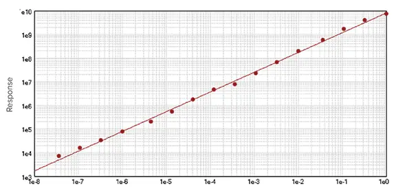
Figure 1. Example of a linear curve fit. Image Credit: Molecular Devices UK Ltd

Nonlinear regression 

Nonlinear datasets are better described with logistic regression, which captures more complex relationships. The objective is to determine the parameter values that minimize the deviations between measured and expected values. 

Choosing the right fit depends on recognizing how model curves compare to the actual data.² 

SoftMax Pro includes 17 nonlinear regression curve-fitting methods: quadratic, cubic, quartic, log-logit, cubic spline, exponential, rectangular hyperbola (with and without a linear term), two-parameter exponential, bi-exponential, bi-rectangular hyperbola, two-site competition, Gaussian, Brain-Cousens, 4P, 5P, and 5P alternate. 

To ensure optimal curve-fitting, SoftMax Pro has been employed with the Levenberg-Marquardt algorithm, the most widely used iterative procedure for nonlinear curve-fitting.

The most widely used nonlinear models are the four- and five-parameter logistic fits, both producing the familiar S-shaped curve (Figure 2). These models require a minimum of four data points for the 4P curve fit model and five for the 5P curve fit model. However, using at least six points for these regression types allows for a more accurate fit.¹ The following equation describes the 4P curve fit: 

y = ((A - D) / (1+ ((x/C)^B))) + D

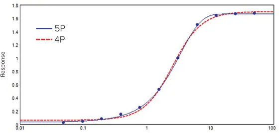
Figure 2. Concentration-response curve fitted with the 4P and the 5P curve fit models for comparison. Although the 4P model gives a smooth symmetrical curve, data are clearly asymmetrical. Therefore, the 5P model gives a better fit. Image Credit: Molecular Devices UK Ltd

Where y is the response, D is the response at infinite analyte concentration, A is the response at zero analyte concentration, x is the analyte concentration, C is the inflection point (EC₅₀/IC₅₀), and B is the slope factor. 

The response increases with the concentration of AD. The 4P model is a symmetrical function: each half mirrors the other, with the EC₅₀/IC₅₀ located in the middle. 

However, certain immuno- and bio-assay data sets are not symmetrical and require additional flexibility. In cases where data are skewed, the 5P model provides extra flexibility by allowing for asymmetry (Figure 2). The general equation is as follows: 

y = ((A - D) / (1 + ((x/C)^B)) ^G) + D

The asymmetry parameter allows variation between each half of the curve. However, when the level of asymmetry is minimal, the 4P curve fit model is recommended, particularly when Parallel Line Analysis (PLA) is employed in the assay. 

Choosing the best curve fit. 

Assessing the overall quality of the curve fit, especially the standard curve, is essential for obtaining precise and reliable data. Since assay noise can obscure poor model performance in a single run, multiple experiments are recommended when evaluating a curve fit model. The R² value is often used as an indicator of fit quality, but it is not always reliable on its own. An R² value greater than 0.99 is considered a strong fit. 

However, the R² value can be misleading, especially if the standard deviation varies with sample concentration.³ Ideally, the standard deviation should be consistent at all sample concentrations (homoscedastic data); however, in practice, the standard deviation generally increases with the sample concentration (heteroscedastic data). 

More robust evaluation methods include Sum of Squares Error (SSE) and Akaike’s Information Criterion (AIC). Both methods are similar in that they assess the error between obtained and predicted values based on the selected curve fit model. 

The SSE method, also known as the summed square of residuals method, uses residuals and residual plots (residuals vs. concentration). The residuals represent the differences between the response y and the predicted response ŷ obtained from the selected curve fit model at each concentration: Residual = data – fit = y – ŷ. Residuals represent random errors.⁴ 

A good model produces residuals that scatter randomly around zero, without obvious patterns (Figure 3A). A systematic pattern in the residuals plot (Figure 3B) clearly indicates that the model is a poor fit for the data. 

Residual plots of data fitted to linear and 4P curve models 

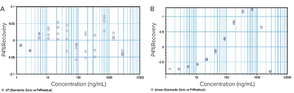
Figure 3. Residual plots of data fitted to linear and 4P curve models. (A) The plotted residuals appear randomly scattered around zero indicating that the 4P model describes the data well. (B) The residuals display a systematic pattern showing that the linear model fits the data poorly. Image Credit: Molecular Devices UK Ltd

The SSE is calculated using the following formula:

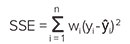
Minimizing the SSE yields a maximum likelihood estimate of the model parameters, assuming the data errors are independent and normally distributed. The optimal curve fit has parameters that produce the smallest SSE. When both models provide a reasonable fit to the data, the plot with the smallest SSE is preferred. 

When the two models are nested and one is a special case of the other, such as a 4P being a special case of a 5P where G = 1, the model with the more detailed equation (i.e., more parameters) is guaranteed to have an SSE less than or equal to the other model. This is because models with more parameters allow more inflection points to fit the data.⁴

Consequently, additional statistical computations, the F test and F probability, are required to identify the model that best fits the data. The F probability applies the F test and the degrees of freedom associated with the curve fit model to assess if the reduction in SSE occurred by chance.

Usually, a probability value under 0.05 (corresponding to 95 % confidence) is used as the threshold, indicating that the model with the most detailed equation yields a superior representation of the data.

The AIC method employs a likelihood statistic to compare the fit quality of the given data for two curve fit models, where one model is a special case of the other. The AIC can be determined using the SSE for data with normally distributed errors as follows:

AIC = n * log (SSE/n) + 2K

Where n represents the sample size and K indicates the number of parameters characterizing the curve. For small sample sizes (i.e., n/K < \~40), the second-order Akaike Information Criterion (AIC_c) should be applied instead:

AIC_c= AIC + 2K ^* (K+1) / (n-K-1)

Where n indicates the sample size and K shows the number of parameters characterizing the curve. 

As the sample size increases, the last term of the AIC_c approaches zero, and the AIC_c tends to yield the same conclusions as the AIC⁵. Both the AIC and AIC_c consider statistical fit quality along with the number of parameters that have to be estimated to achieve this degree of fit. 

The AIC penalizes over-complexity, favoring models that balance accuracy with simplicity. The curve fit with lower AIC or AIC_c values is considered the superior model. That is, the one that provides a good fit of the data with the fewest parameters.⁵ 

Both approaches are beneficial for identifying the curve fit that best represents the data; however, they do not provide a test of a model in the sense of testing a null hypothesis; specifically, they do not provide information about fit quality. If only poor models are considered, the model will logically select the best model among them.

There is an unlimited number of possible models; curve fitting can determine the optimal parameters for a specific model or compare two models, but any candidate models should be based on prior studies and scientific considerations.

After establishing a set of plausible models to interpret the data, and before conducting further analysis, one should assess the fit of the global model, which is defined as the most complex model of the set. The general assumption is that if the global model fits, simpler models will also fit, as they are derived from it.^5,6

Measuring the goodness of the fit

SoftMax Pro 7 includes a new parameter, Independence, which offers a method for assessing the appropriateness of a specific curve fit for the data set. Parameter dependency measures how much one parameter relies on the values of others in the model.

For a curve fit model of two or more parameters, the parameters defining the curve can be either intertwined (the desired case with an independence value of one) or redundant (the worst case with an independence value of zero). 

If a single parameter is altered after fitting the data with the selected curve fit, the curve deviates from the data points. If the values of the other parameters are changed to account for the fixed parameter, and the curve approaches the points, but with a different curve fit from the one originally established, then the parameters are intertwined. 

Conversely, if the curve returns to its original position, then the parameters are redundant. Independence values range from zero to one, with one representing the ideal scenario. To display the independence value in the graph legend, click the curve fit settings icon (Figure 4). The curve fit settings window will appear. Simply select the Statistics tab and click “Calculate Parameter Dependencies”. 

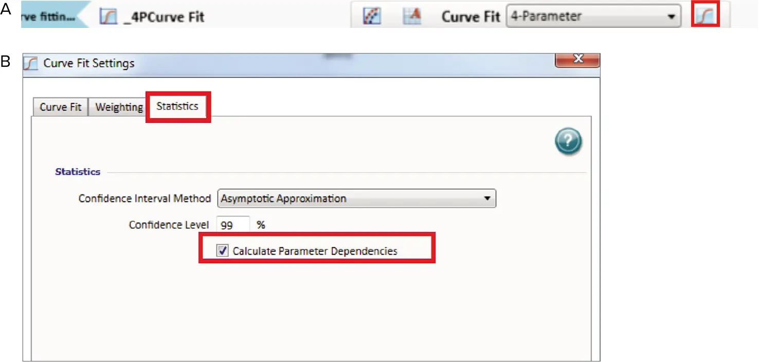
Figure 4. Curve fit display in SoftMax Pro 7. (A) Menu. (B) Curve fit settings. Image Credit: Molecular Devices UK Ltd

The graph legend will now display the independence values for each parameter describing the curve (Figure 5). 

In the graph fit legend displayed in Figure 5, parameter independence is represented by bars with logarithmic scaling. Ten bars indicate a high level of independence. Given that only minute values signal a problem, a nonlinear transformation is applied for this translation. If one or more parameters display few or no bars, the curve fit may be unsuitable for the data set.

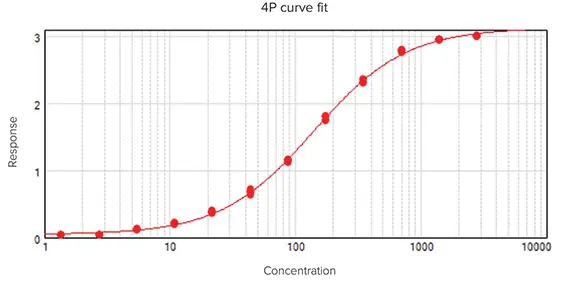
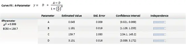
Figure 5. Graph legend showing the parameter independence. The independence is translated into bars, where ten bars indicate a high degree of independence. Image Credit: Molecular Devices UK Ltd

For sigmoidal data with clear upper and lower limits, a 4P model typically provides the best fit. Conversely, when one or both asymptotes are absent, the A or D parameter will show few bars, indicating that dependable values cannot be inferred from the data set. 

Protocol available: Curve Fitting Evaluation 

A protocol titled Curve Fitting Evaluation has been developed in SoftMax Pro to automatically determine the SSE, F probability, and AIC_c values upon data input. A results section has been implemented that contains all relevant computations along with the curve fit conclusion based on both the SSE and AIC_c methods (Figure 7). The protocol is available for download via the SoftMax Pro Protocol Home. 

In the following example, data were fitted to a 4P (Figure 6A) and a 5P (Figure 6B) curve fit model, yielding an R² value of 1. All results and computations are summarized in Figure 7.

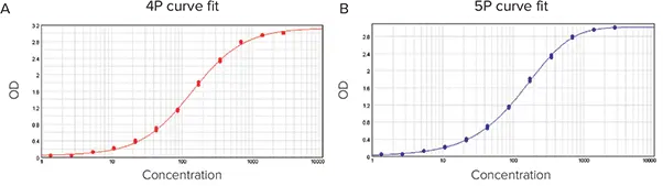
Figure 6. Data fitted into curve models. (A) 4P curve fit. (B) 5P curve fit. Image Credit: Molecular Devices UK Ltd

Figure 7. SSE and AIC_c tests. Results of data fitted into 4P and 5P curve models using the Curve Fitting Evaluation protocol. Image Credit: Molecular Devices UK Ltd

The SSE method demonstrated that the 5P curve fit model was superior to the 4P, with SSE values of 0.058 for the 4P and 0.027 for the 5P curve fit model. 

The issue was that the 4P curve fit model represented a specific case of the 5P curve fit model (4P is 5P where G=1). Therefore, the 5P curve fit model was at least as good as the 4P model. Further statistical analysis was required. In this example, the F test (61.539) and F probability (0.000) verified that the 5P curve fit model more accurately represented the data than the 4P curve fit model. 

The AIC_c method also demonstrated that the 5P fit the data more effectively than the 4P curve fit model, with AIC_c values of -405.365 for the 4P curve fit model and -447.945 for the 5P curve fit model. 

Lastly, the residual plot exhibited residuals randomly scattered around the zero line, confirming that both curve fit models were accurate fits (Figure 8). Collectively, the test methods demonstrated that the 5P curve fit model fit the data more effectively. 

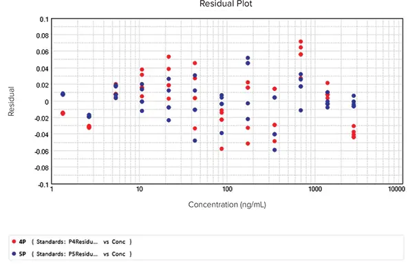
Figure 8. Residual plot for data fitted into 4P and 5P curve models. Image Credit: Molecular Devices UK Ltd

Summary 

SoftMax Pro 7 offers a broad selection of mathematical models, including the popular 4P and 5P curve fit models. The R² value may be a poor indicator of curve fit quality, especially for heteroscedastic data. 

Using SSE, F probability, and AIC_c together offers a more confident way to judge fit quality. However, the first step is to ensure that both models fit the data with reasonable values and are scientifically sound. 

SoftMax Pro 7 now calculates parameter dependency, giving researchers a clearer view of curve fit quality. The resulting parameter independence value is visualized in the graph legend to streamline data interpretation. 

References and further reading: 

1. Davis, D. et al. (2021) Principles of curve fitting for multiplex sandwich immunoassays (tech note), Bio-Plex. tech note. Bio-Rad Laboratories, Inc. https://geiselmed.dartmouth.edu/dartlab/wp-content/uploads/sites/22/2017/05/Bio-RadTechNote2861_principles_of_curve_fitting.pdf. 
2. M. Ledvij (2003). Curve fitting made easy. Industrial Physicist, (online) 9(2), pp.24–27. Available at: https://www.researchgate.net/publication/285760926_Curve_fitting_made_easy.
3. Kiser, M.M. and Dolan, J.W. (2004). Selecting the Best Curve Fit. LCGC North America, (online) 17(3), pp.138–143. Available at: https://www.researchgate.net/publication/281595912_Selecting_the_Best_Curve_Fit.  
4. Gottschalk, P.G. and Dunn, J.R. (2005). The five-parameter logistic: A characterization and comparison with the four-parameter logistic. Analytical Biochemistry, 343(1), pp.54–65. https://doi.org/10.1016/j.ab.2005.04.035. 
5. Burnham, K.P. and Anderson, D.R. eds., (2004). Model Selection and Multimodel Inference. New York, NY: Springer New York. https://doi.org/10.1007/b97636. 
6. Cooch EG and White GC. (2001) Program MARK: Analysis of data from marked individuals, a ‘gentle introduction’. www.phidot.org/software/mark/docs/book.

About Molecular Devices UK Ltd

Molecular Devices is one of the world’s leading providers of high-performance bioanalytical measurement systems, software, and consumables for life science research, pharmaceutical, and biotherapeutic development. Included within a broad product portfolio are platforms for high-throughput screening, genomic and cellular analysis, colony selection, and microplate detection. These leading-edge products enable scientists to improve productivity and effectiveness, ultimately accelerating research and the discovery of new therapeutics. Molecular Devices is committed to the continual development of innovative solutions for life science applications. The company is headquartered in Silicon Valley, California, with offices around the globe. For more information, please visit www.moleculardevices.com. 

Sponsored Content Policy: News-Medical.net publishes articles and related content that may be derived from sources where we have existing commercial relationships, provided such content adds value to the core editorial ethos of News-Medical.Net which is to educate and inform site visitors interested in medical research, science, medical devices and treatments.